The other day, I wondered how sorting algorithms actually work. This prompted me to take a closer look at them. In the process, I learned a lot of interesting things that I would like to share with you. In this article, I will introduce various sorting algorithms and explain how they work using Python code and illustrative graphics. I will look at well-known algorithms such as bubble sort and quick sort, as well as more unusual ones such as bogosort. I will also discuss the speed of the algorithms and find out which ones are suitable for which use cases.
 All sorting processes in comparison
Why are sorting algorithms important?
Sorting algorithms play an important role in computer science. They are used wherever data needs to be organized, e.g., in databases, search engines, or when processing large amounts of data. Efficient sorting algorithms can significantly improve the speed of applications. In the next section, I will first create a data set, which I will then process using various sorting algorithms.
The data set to be sorted
It will be a simple data set that should be easy to visualize. Specifically, it will consist of a certain number of integer values that should be randomized each time. A visualization will follow shortly.
import matplotlib.pyplot as plt
import matplotlib.cm as cm
import random
import os
import time
random.seed(42)
n = 50
dataset = random.sample(range(1, n+1), n)Then I define a function that I will use more often to visualize the sorting.
cmap = cm.get_cmap("YlGnBu") # Color gradient from yellow to green to blue
def update_chart(data, iteration, xlim, ylim, folder_name, name = "Dataset",):
i = len(data)
colors = [cmap(x/i) for x in data]
plt.bar(range(1, i+1), data, color=colors)
plt.xlim(xlim)
plt.ylim(ylim)
plt.xticks([])
plt.yticks([])
if not os.path.exists(folder_name):
os.makedirs(folder_name)
if name == "Start":
plt.title(f'Start configuration')
plt.savefig(f'{folder_name}/{name}.png')
else:
plt.title(f'{name} - Step {iteration}')
plt.savefig(f'{folder_name}/{name}_Iteration_{iteration:04d}.png') # Speichere den Plot als PNG-Datei
plt.close()Theoretically, of course, you don’t have to save the plot. However, it is very helpful for my workflow when creating this post.And then the function is called for the first time.
update_chart(dataset, 1, xlim=[0, n+1], ylim=[0, n+.5], folder_name="Sorting Algorithms", name="Start")Next, I call up the plot again. Here you can see the unsorted data set, consisting of integer values.
image = plt.imread("SortingAlgorithms/Start.png")
# Show the image
plt.imshow(image)
plt.axis("off")
plt.show()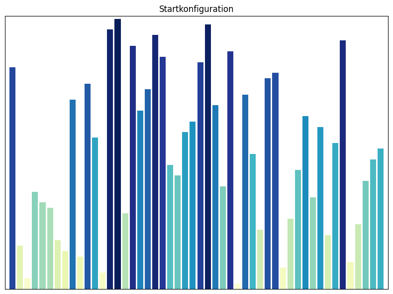 Start configuration: Every sorting algorithm starts with this data set
Sorting algorithms
In the following, I will introduce a few sorting algorithms that, as far as I know, are among the most common. I will say a few words about each algorithm and then implement it. Since I also want to visualize the sorting process, I will program a few additional lines that are unnecessary for the algorithm. I have tried to keep everything consistent, but because this post was written with a few breaks, there are probably a few outliers here and there.
Bubble Sort
Bubble sort is a simple comparison sorting algorithm that repeatedly compares adjacent elements and swaps them if they are in the wrong order. This process continues until no more swaps are necessary, which means that the array is sorted. The name “bubble sort” comes from the fact that smaller elements rise to the top like bubbles in water, just as the elements to be sorted rise to the top.
- How it works: In each pass, the array is traversed from start to finish. Two adjacent elements are compared at a time. If the left element is greater than the right, they are swapped. At the end of the first pass, the largest element is at the end of the array. In the second pass, the second largest element is found, and so on.
- Time complexity: The time complexity of bubble sort is on average and in the worst case, where is the number of elements in the array. For large data sets, bubble sort can therefore be very inefficient and is often replaced in practice by faster sorting algorithms such as quick sort, merge sort, or heap sort.
- Special features: Bubble sort is easy to understand and implement, but inefficient for large data sets. It is a stable sorting algorithm, i.e., the relative order of equal elements is preserved.
 Bubble sort sorting process
Theoretically, the data set to be sorted already exists. For the sake of completeness, I will still generate it each time.
n = 50
dataset = random.sample(range(1, n+1), n)Next, I define the function with the sorting algorithm.
def bubble_sort(data):
"""
Implements the bubble sort algorithm and saves snapshots of the array after each swap. This algorithm
sorts a list of numbers by repeatedly going through the list, comparing each pair of adjacent
elements, and swapping them if they are in the wrong order.
Args:
data (list): The list of numbers to be sorted.
Returns:
sorted_datasets (list): A list containing the state of the sorted list after each swap.
"""
def swap(i, j):
"""
Helper function for the bubble sort algorithm. It swaps the elements at positions i and j.
Args:
i (int): The index of the first element.
j (int): The index of the second element.
"""
data[i], data[j] = data[j], data[i] # Swap the elements at positions i and j
sorted_datasets = [] # Initialize an empty list to store the sorted datasets
n = len(data) # The number of elements in the dataset.
for i in range(n): # For each element in the dataset.
for j in range(0, n-i-1): # For each element that is not yet sorted.
if data[j] > data[j+1]: # If the current element is greater than the next element
swap(j, j+1) # Swap the two elements
sorted_datasets.append(data[:]) # Save the current state of the dataset
return sorted_datasets # Return the list of sorted datasetsFollowing the definition of the sorting algorithms in this post, each of these algorithms is executed. As each sorting step is run, a visualization function is called that saves the current state of the sorting process as a PNG image. At the end of the post, a GIF is created from these images for each sorting process, also using Python. The first of these GIFs can already be seen above in the post.
for i, data in enumerate(bubble_sort(dataset)):
update_chart(data, i+1, xlim=[0, n+1], ylim=[0, n+.5], folder_name="SortingAlgorithms/bubble_sort", name="Bubble Sort")I will do the same for the other sorting processes as I have done here for bubble sort, but I will not comment on them again.
Insertion Sort
Insertion sort builds the sorted array step by step by taking each element from the unsorted part and inserting it in the correct place in the sorted part.
- How it works: The algorithm starts with the second element and compares it with the first element. If it is smaller, it is inserted before the first element. Then the third element is taken and compared with the first two, and so on. At the end of each step, the left part of the array is sorted.
- Time complexity: on average and in the worst case. However, insertion sort is more efficient than bubble sort if the array is already partially sorted. In this case, each element only needs to be moved a short distance to get to the correct position. Therefore, the time complexity of insertion sort can be close to in such cases. This only applies to partially sorted arrays. For randomly sorted arrays, the time complexity of insertion sort is still .
- Special features: Insertion sort is an in-place algorithm, i.e., it does not require additional storage space. It is easy to implement and efficient for small data sets or almost sorted data.
 Insertion sort sorting process
n = 50
dataset = random.sample(range(1, n+1), n)def insertion_sort(data):
"""
Implements the insertion sort algorithm and saves snapshots of the array after each insertion. This algorithm
sorts a list of numbers by inserting each element into the correct position in the already sorted subset
of the list.
Args:
data (list): The list of numbers to be sorted.
Returns:
sorted_datasets (list): A list containing the state of the sorted list after each insertion.
"""
def insert(j, key):
"""
Helper function for the insertion sort algorithm. It moves elements to the right and inserts the
key element in the correct position.
Args:
j (int): The index where the key element should be inserted.
key (int): The key element to be inserted.
"""
while j >= 0 and data[j] > key: # As long as we are not at the beginning of the array and the current element is greater than the key element
data[j+1] = data[j] # Move the current element to the right
j -= 1 # Go to the next element on the left
data[j+1] = key # Insert the key element in the correct position
sorted_datasets = [] # Initialize an empty list to store the sorted datasets
for i in range(1, len(data)): # Start at the second position in the array
insert(i - 1, data[i]) # Insert the element `data[i]` in the correct position
sorted_datasets.append(data[:]) # Save the current state of the array
return sorted_datasets # Return the list of sorted datasetsfor i, data in enumerate(insertion_sort(dataset)):
update_chart(data, i+1, xlim=[0, n+1], ylim=[0, n+.5], folder_name="Sorting Algorithms/insertion_sort", name="Insertion Sort")Selection Sort
In each pass, Selection Sort finds the smallest element in the unsorted part of the array and swaps it with the first element of the unsorted part.
- How it works: The algorithm goes through the array and finds the smallest element. This is swapped with the first element. The process is then repeated for the remaining unsorted part of the array.
- Time complexity: in all cases. The number of comparisons is always the same, regardless of the order of the elements.
- Special features: Selection sort is easy to understand and implement, but it is not efficient for large data sets. One advantage of selection sort over some other sorting algorithms, such as bubble sort, is that it minimizes the number of swaps, which can be useful when swapping elements is an expensive operation.
 Selection sort process
n = 50
dataset = random.sample(range(1, n+1), n)
def selection_sort(data):
"""
Implements the selection sort algorithm and stores snapshots of the array after each swap. This algorithm
sorts a list of numbers by finding the smallest element and swapping it with the first element,
then finding the second smallest element and swapping it with the second element, and so on.
Args:
data (list): The list of numbers to be sorted.
Returns:
sorted_datasets (list): A list containing the state of the sorted list after each swap.
"""
def find_min_index(start_index):
"""
Helper function for the selection sort algorithm. It finds the index of the smallest element starting from the
given start index.
Args:
start_index (int): The start index for the search.
Returns:
min_index (int): The index of the smallest element starting from the start index.
"""
min_index = start_index
for j in range(start_index+1, len(data)):
if data[j] < data[min_index]:
min_index = j
return min_index
sorted_datasets = [] # Initialize an empty list to store the sorted datasets
for i in range(len(data)-1): # For each element in the dataset, except the last
min_index = find_min_index(i) # Find the index of the smallest element from the current index
data[i], data[min_index] = data[min_index], data[i] # Swap the current element with the smallest element
sorted_datasets.append(data[:]) # Save the current state of the dataset
return sorted_datasets # Return the list of sorted datasetsfor i, data in enumerate(selection_sort(dataset)):
update_chart(data, i+1, xlim=[0, n+1], ylim=[0, n+.5], folder_name="SortingAlgorithms/selection_sort", name="Selection Sort")Merge Sort
Merge sort is a “divide and conquer” algorithm that recursively divides the array into two halves, sorts each half, and then merges the sorted halves.
- How it works: The array is halved until only single elements remain. These are trivially sorted. Then the single elements are merged into sorted pairs, then pairs into groups of four, and so on, until the entire array is sorted.
- Time complexity: The time complexity of merge sort is in all cases, since the array is halved in each step and then the two halves are merged in time. This makes merge sort efficient for large data sets.
- Special features: Merge sort is a stable sorting algorithm, which means that equal elements in the sorted output have the same relative order as in the input. A disadvantage of merge sort is that it requires additional memory to store the two halves during merging.
Merge sort sorting process
n = 50
dataset = random.sample(range(1, n+1), n)import itertools
def merge_sort(data):
"""
Implements the merge sort algorithm and stores snapshots of the array after each merge. This algorithm
sorts a list of numbers by dividing it into two halves, sorting each half, and then merging the sorted
halves.
Args:
data (list): The list of numbers to be sorted.
Returns:
steps (list): A list containing the state of the sorted list after each merge.
"""
steps = [] # List for storing intermediate steps
def merge(left, right, start):
"""
Helper function for the merge sort algorithm. It merges two sorted lists and stores
snapshots of the array after each merge.
Args:
left (list): The left sorted list.
right (list): The right sorted list.
start (int): The start index for merging in the original array.
Returns:
result (list): The merged and sorted list.
"""
result = [] # Result list
i = j = 0 # Initialize the indexes for the left and right lists
# Iterate through both lists and add the smaller element to the result list
while i < len(left) and j < len(right):
if left[i] < right[j]:
result.append(left[i])
i += 1
else:
result.append(right[j])
j += 1
# Update the corresponding part of the original array and save the step
data[start:start+len(result)] = result
steps.append(list(data))
# Add the remaining elements from left or right
for value in itertools.chain(left[i:], right[j:]):
result.append(value)
data[start:start+len(result)] = result
steps.append(list(data))
return result # Return the sorted list
def sort(data, start=0):
"""
Helper function for the merge sort algorithm. It splits the array into two halves, sorts each half,
and then merges them together.
Args:
data (list): The array to be sorted.
start (int): The starting index for sorting in the original array.
Returns:
list: The sorted list.
"""
if len(data) <= 1: # If the list contains only one element, it is already sorted
return data
mid = len(data) // 2 # Find the middle index
left = data[:mid] # Split the list into two halves
right = data[mid:]
# Sort both halves and merge them
return merge(sort(left, start), sort(right, start + mid), start)
sort(data) # Start the sorting process
return steps # Return the list of intermediate stepsfor i, data in enumerate(merge_sort(dataset)):
update_chart(data, i+1, xlim=[0, n+1], ylim=[0, n+.5], folder_name="SortingAlgorithms/merge_sort", name="Merge Sort")Quick Sort
Quick Sort is another “divide and conquer” algorithm. It selects an element as a “pivot” and partitions the array into two sub-areas: elements smaller than the pivot and elements larger than the pivot. The sub-areas are then sorted recursively.
- How it works: The algorithm selects an element as a “pivot” and divides the array into two sub-areas: elements smaller than the pivot and elements larger than the pivot. These sub-areas are then sorted recursively. The choice of pivot can greatly influence the efficiency of the algorithm.
- Time complexity: The average time complexity of Quick Sort is , but in the worst case (if the smallest or largest element is chosen as the pivot), it can increase to $O(n^2) in the worst case (if the smallest or largest element is chosen as the pivot).
- Special features: Quick Sort is an in-place algorithm, which means that it does not require any additional storage space. In practice, it is often faster than Merge Sort, even though its time complexity is higher in the worst case. One disadvantage of Quick Sort is that it is not stable, i.e., equal elements may change their relative order during sorting.
Quicksort sorting process
n = 50
dataset = random.sample(range(1, n+1), n)def quick_sort_visualized(arr):
"""
Implements the Quick Sort algorithm and saves snapshots of the array after each swap. This algorithm
sorts a list of numbers by selecting a "pivot" element and arranging all elements that are smaller
to the left of the pivot and all elements that are larger to the right of the pivot. This process is then
recursively applied to the left and right halves of the array.
Args:
arr (list): The list of numbers to be sorted.
Returns:
snapshots (list): A list containing the state of the sorted list after each swap.
"""
snapshots = [arr[:]] # Initial snapshot before sorting begins
def _quick_sort(arr, low, high):
"""
Helper function for the quick sort algorithm. It performs the actual sorting process and calls
itself recursively on the left and right halves of the array.
Args:
arr (list): The array to be sorted.
low (int): The starting index of the part of the array to be sorted.
high (int): The end index of the part of the array to be sorted.
"""
if low < high:
pivot_index = partition(arr, low, high)
snapshots.append(arr[:]) # Snapshot after each swap operation
_quick_sort(arr, low, pivot_index - 1)
_quick_sort(arr, pivot_index + 1, high)
def partition(arr, low, high):
"""
Helper function for the quick sort algorithm. It selects a pivot element and arranges all elements that are
smaller to the left of the pivot and all elements that are larger to the right of the pivot.
Args:
arr (list): The array to be sorted.
low (int): The starting index of the part of the array to be sorted.
high (int): The ending index of the part of the array to be sorted.
Returns:
int: The index of the pivot element after partitioning.
"""
pivot = arr[high]
i = low - 1
for j in range(low, high):
if arr[j] <= pivot:
i += 1
arr[i], arr[j] = arr[j], arr[i]
snapshots.append(arr[:]) # Snapshot nach jedem Swap
arr[i + 1], arr[high] = arr[high], arr[i + 1]
snapshots.append(arr[:]) # Snapshot nach dem finalen Swap
return i + 1
_quick_sort(arr, 0, len(arr) - 1)
return snapshotsfor i, data in enumerate(quick_sort_visualized(dataset)):
update_chart(data, i+1, xlim=[0, n+1], ylim=[0, n+.5], folder_name="SortingAlgorithms/quick_sort", name="Quicksort")Heap Sort
Heap Sort uses a special data structure called a heap to sort the array. A heap is a binary tree in which each node is larger (or smaller, depending on the implementation) than its children.
-
How it works: The heap sort algorithm begins by converting the array into a heap. Then, the largest element (the root of the heap) is removed and placed at the end of the array. This process is repeated until the entire array is sorted. After each removal, the heap is restored to maintain the heap property.
-
Time complexity: The time complexity of heap sort is in all cases. This is because creating the heap takes time and removing each element takes time.
-
Special features: Heap sort is an in-place algorithm, which means it does not require additional storage space. It guarantees a time complexity of , regardless of the arrangement of the elements. A disadvantage of heap sort is that it is more complex to implement than other sorting algorithms such as quick sort or merge sort.
Heapsort sorting process
dataset = random.sample(range(1, n+1), n)def heapify(arr, n, i, snapshots):
"""
Helper function for the heap sort algorithm. It takes an array and transforms it into a heap by
ensuring that the element at position i is greater than its children. If this is not the case,
the element is swapped with the largest child and the process is continued recursively.
Args:
arr (list): The array to be converted into a heap.
n (int): The number of elements in the array.
i (int): The index of the element to be "heapified."
snapshots (list): A list that stores the state of the array after each step.
"""
def heap_sort(arr):
"""
Implements the heap sort algorithm. This algorithm sorts a list of numbers by first converting it
into a heap and then removing the elements of the heap in descending order and
appending them to the end of the list.
Args:
arr (list): The list of numbers to be sorted.
Returns:
snapshots (list): A list containing the state of the sorted list after each step.
"""
n = len(arr)
snapshots = [arr.copy()] # Save initial state
# Create heap (bottom-up)
for i in range(n // 2 - 1, -1, -1):
heapify(arr, n, i, snapshots)
# Remove one element at a time from the heap and place it in the correct position
for i in range(n - 1, 0, -1):
arr[i], arr[0] = arr[0], arr[i] # Swap root with last element
snapshots.append(arr.copy()) # Save snapshot
heapify(arr, i, 0, snapshots) # Restore heap
return snapshotsfor i, data in enumerate(heap_sort(dataset)):
update_chart(data, i+1, xlim=[0, n+1], ylim=[0, n+.5], folder_name="SortingAlgorithms/heap_sort", name="Heapsort")Radix Sort
Radix Sort sorts numbers by their individual digits, starting with the least significant digit (ones place).
- How it works: Radix Sort sorts numbers based on their individual digits, starting with the least significant digit (ones place). In each pass, the numbers are sorted into “buckets” based on the digit at the current position. The buckets are then reassembled in the correct order. This process is repeated for each digit until all digits are sorted.
- Time complexity: The time complexity of radix sort is , where n is the number of elements and k is the maximum number of digits. This makes radix sort very efficient when the number of digits is limited.
- Special features: Radix sort is particularly efficient for integers with a limited number of digits. It is not a comparison-based algorithm, but uses the distribution of digits to sort the numbers. This distinguishes radix sort from many other sorting algorithms that are based on comparisons.
Radix sort sorting process
n = 50
dataset = random.sample(range(1, n+1), n)
def flatten_and_fill(buckets, arr_length):
"""
Flattens a list of lists (buckets) and fills the resulting list with zeros until it reaches the
specified length. This function is used in sorting algorithms that use buckets to sort elements, such as the radix sort algorithm.
Args:
buckets (list): A list of lists to be flattened.
arr_length (int): The desired length of the resulting list.
Returns:
list: A flattened list filled with zeros until it reaches the specified length.
"""
flattened = [item for sublist in buckets for item in sublist]
return flattened + [0] * (arr_length - len(flattened))
def radix_sort(arr):
"""
Implements the radix sort algorithm. This algorithm sorts a list of numbers by sorting them
based on the individual digits from left to right. The algorithm uses a
bucket sort strategy to sort the numbers into "buckets" based on the current digit being
sorted.
Args:
arr (list): The list of numbers to be sorted.
Returns:
snapshots (list): A list of lists containing the state of the sorted list after each step.
"""
max_value = max(arr)
exp = 1
snapshots = [arr.copy()] # Initial state
while max_value // exp > 0:
buckets = [[] for _ in range(10)]
for num in arr:
digit = (num // exp) % 10
buckets[digit].append(num)
snapshots.append(flatten_and_fill(buckets, len(arr))) # Save the snapshot
arr = [num for bucket in buckets for num in bucket]
exp *= 10
return snapshotsfor i, data in enumerate(radix_sort(dataset)):
update_chart(data, i+1, xlim=[0, n+1], ylim=[0, n+.5], folder_name="Sorting Algorithms/radix_sort", name="Radix Sort")Bogo Sort
Bogo Sort is an inefficient and non-deterministic sorting algorithm. It works by randomly shuffling the array and then checking whether it is sorted. This process is repeated until the array is randomly sorted into the correct order. For this reason, I have reduced the size of the data set.
- How it works: Bogo Sort randomly shuffles the array and then checks whether it is sorted. This process is repeated until the array is randomly sorted into the correct order. There is no guarantee how long this will take. In the worst case, it can take an infinite amount of time.
- Time complexity: The time complexity of Bogo Sort is infinite on average and in the worst case, as there is no guarantee that the algorithm will ever end. This makes Bogo Sort extremely inefficient.
- Special features: Bogo Sort is an example of an extremely inefficient and impractical sorting algorithm. It is often used as a humorous example of a bad algorithm.
Bogosort sorting process
n = 5 # Reduced size of the data set
dataset = random.sample(range(1, n+1), n)def bogo_sort(data):
"""
Implements the Bogo sort algorithm. This algorithm sorts a list by repeatedly randomly
shuffling the elements until the list is sorted. It is a very inefficient sorting algorithm with an
average time complexity of O((n+1)!), where n is the number of elements in the list.
Args:
data (list): The list of numbers to be sorted.
Returns:
steps (list): A list containing the state of the sorted list after each step.
"""
steps = [] # Initialize a list to store the steps of the sorting process
# Repeat the process until the array is sorted
while not all(data[i] <= data[i+1] for i in range(len(data)-1)):
steps.append(list(data)) # Add the current state of the array to the steps
random.shuffle(data) # Shuffle the array randomly
steps.append(list(data)) # Add the final sorted array to the steps
return steps # Return the list of stepsfor i, data in enumerate(bogo_sort(dataset)):
update_chart(data, i+1, xlim=[0, n+1], ylim=[0, n+.5], folder_name="SortingAlgorithms/bogo_sort", name="Bogosort")Sleep Sort
Sleep Sort is an unconventional and inefficient sorting algorithm based on the idea that each thread “sleeps” for a time proportional to the value of the element. Again, I will refrain from using a large data set.
- How it works: Sleep Sort starts a thread for each element in the array. Each thread “sleeps” for a time proportional to the value of the element. When a thread wakes up, it outputs its element. Since threads with smaller values wake up first, the elements are output in sorted order.
- Time complexity: The time complexity of Sleep Sort is , where is the largest element in the array. This makes Sleep Sort inefficient for large amounts of data or arrays with very large values.
- Special features: Sleep Sort is not deterministic, as the order of output may vary for identical elements. It is more of a curiosity and not intended for practical use.
Sleepsort sorting process
n = 50
dataset = random.sample(range(1, n+1), n)import time
import threading
def sleep_sort(data):
"""
Sorts a list of numbers using the sleep sort algorithm. This algorithm uses multithreading
to sort the numbers. Each number in the list is assigned to a separate thread. Each thread
waits for a period of time proportional to the value of the number before adding the number to the sorted list.
Args:
data (list): The list of numbers to be sorted.
Returns:
all_steps (list): A list containing the state of the sorted list after each step.
"""
sorted_data = [0] * len(data) # Initialize sorted_data with zeros
all_steps = [] # Initialize the list to store all steps
index = 0 # Initialize the index
def sleep_func(x):
nonlocal index # Declare index as nonlocal
time.sleep(x/10) # Let the thread sleep for a time proportional to the value of x
sorted_data[index] = x # Insert the element at the current index
index += 1 # Increment the index
all_steps.append(list(sorted_data)) # Add the current state of sorted_data to all_steps
threads = []
for num in data:
t = threading.Thread(target=sleep_func, args=(num,)) # Create a thread for each number in the array
threads.append(t)
t.start() # Start the thread
for t in threads:
t.join() # Wait until all threads have finished
return all_steps # Return the list of all stepsfor i, data in enumerate(sleep_sort(dataset)):
update_chart(data, i+1, xlim=[0, n+1], ylim=[0, n+.5], folder_name="SortingAlgorithms/sleep_sort", name="Sleepsort")There are many other sorting algorithms. And I may add one or two more.
Creating GIFs
The following lines contain the code I used to create the GIFs. Of course, much of it could be programmed in a more elegant and streamlined way, but I think it’s still readable as it is.
def get_subfolders(folder_path):
    """
    Retrieves the subfolders in the specified folder.
    Parameters:
        folder_path (str): The path to the folder from which to retrieve the subfolders.
    Returns:
        list: A list of paths to the subfolders in the specified folder.
    """

    return [f.path for f in os.scandir(folder_path) if f.is_dir()]
def get_images(subfolder, max_image_width, max_image_height):
"""
Retrieves and resizes images from a specified subfolder.
Parameters:
subfolder (str): The path to the subfolder containing the images.
max_image_width (int): The maximum width to which the images will be resized.
max_image_height (int): The maximum height to which the images will be resized.
Returns:
list: A list of numpy arrays representing the resized images.
"""
png_files = sorted(glob.glob(os.path.join(subfolder, "*.png")))
return [np.array(Image.fromarray(imageio.imread(png_file)[..., :3]).resize((max_image_width, max_image_height))) for png_file in png_files]def create_final_gif_image(i, gif_images, num_gifs_down, num_gifs_across, max_image_height, max_image_width):
"""
Creates a single frame for the final GIF.
Parameters:
i (int): The index of the current frame.
gif_images (list): A list of lists containing the images for each GIF.
num_gifs_down (int): The number of GIFs to be arranged vertically in the final GIF.
num_gifs_across (int): The number of GIFs to be arranged horizontally in the final GIF.
max_image_height (int): The maximum height of the images to be included in the GIF.
max_image_width (int): The maximum width of the images to be included in the GIF.
Returns:
final_gif_image (numpy.ndarray): A 3D numpy array representing the final GIF image for the current frame.
"""
final_gif_image = np.zeros((max_image_height * num_gifs_down, max_image_width * num_gifs_across, 3), dtype=np.uint8)
for j in range(num_gifs_down):
for k in range(num_gifs_across):
images = gif_images[j * num_gifs_across + k]
if i < len(images):
final_gif_image[j * max_image_height:(j + 1) * max_image_height, k * max_image_width:(k + 1) * max_image_width] = images[i]
else:
final_gif_image[j * max_image_height:(j + 1) * max_image_height, k * max_image_width:(k + 1) * max_image_width] = images[-1]
return final_gif_imagedef create_final_gif(folder_path, num_gifs_across, num_gifs_down, max_image_width, max_image_height, output_file):
"""
Creates a final GIF from images in the subfolders of the given folder.
Parameters:
folder_path (str): The path to the folder containing the subfolders with images.
num_gifs_across (int): The number of GIFs to be arranged horizontally in the final GIF.
num_gifs_down (int): The number of GIFs to be arranged vertically in the final GIF.
max_image_width (int): The maximum width of the images to be included in the GIF.
max_image_height (int): The maximum height of the images to be included in the GIF.
output_file (str): The path to the output file where the final GIF will be saved.
Returns:
None
"""
subfolders = get_subfolders(folder_path)
gif_images = [get_images(subfolder, max_image_width, max_image_height) for subfolder in subfolders]
final_gif_images = [create_final_gif_image(i, gif_images, num_gifs_down, num_gifs_across, max_image_height, max_image_width) for i in range(max(len(images) for images in gif_images))]
imageio.mimsave(output_file, final_gif_images, duration=0.5)create_final_gif(
folder_path="Sorting algorithms",
num_gifs_across=3,
num_gifs_down=3,
max_image_width=200,
max_image_height=200,
output_file="final.gif")