The Transformer Architecture - Fundamentals and Applications

In this and the following article, I would like to develop a basic understanding of the Transformer architecture and its application in more or less modern language models. The focus will be on the attention mechanism, which is ultimately the core component of this architecture.

A paper I read on this topic is from 2023 and therefore old hat for many, but I have not yet looked into it in detail: Attention is All You Need.

I will begin by demonstrating the generation of text sequences using a practical example with the DistilGPT-2 model. This introduction is intended to illustrate the basic functionality and challenges of statistical text generation. I will then discuss the concepts of tokens and embeddings and attempt to explain them in more detail, as they are essential for language processing by GPTs.

Building on this, I will attempt to explain the attention mechanism in detail, using both theoretical principles and practical examples to visualize attention patterns. The goal is to clarify how the mechanism works and its significance in texts. Let’s start at the beginning…

DistilGPT-2

What is DistilGPT-2?

DistilGPT-2 is a compressed and more efficient version of the well-known language model GPT-2. It was specifically developed to reduce model size and computational effort. This makes it ideal for use on resource-constrained devices such as mobile devices or embedded systems.

This reduction was achieved through a process known as knowledge distillation. This is a training method that transfers knowledge and skills from a larger model (in this case GPT-2) to a smaller model. This results in a smaller number of parameters, which in turn reduces storage space requirements and computing power requirements. This makes DistilGPT-2 ideal for demonstration purposes: you can easily explain and visualize the basics without relying on a particularly powerful computer. A standard laptop is perfectly adequate for experimenting with the model. Of course, this compression also has its disadvantages. It is possible that the model will lose accuracy when performing complex tasks. Its ability to generate long and coherent texts is also limited, as is its linguistic diversity. However, for the applications shown here, this is an acceptable compromise.

Tokens and embeddings – the building blocks

The following is a brief introduction to the building blocks of language models. More detailed information can be found under Tokenization and Embeddings and similarity metrics.

Tokens and Tokenization

Tokens are the basic units into which a language model breaks down text. This process is called Tokenization. Let’s imagine this with a concrete example. We will use the distilgpt2 tokenizer for this.

We import our dependencies and then load the distilgpt2 model and the associated tokenizer. The tokenizer is an essential component because it converts the input text into a numerical representation (token IDs) that the model can work with.

import torch
from transformers import GPT2Tokenizer, GPT2LMHeadModel
 
tokenizer = GPT2Tokenizer.from_pretrained("distilgpt2")
model = GPT2LMHeadModel.from_pretrained("distilgpt2")

Now we define our example sentence. This sentence is converted by the tokenizer into a sequence of token IDs. These IDs are the numerical representation of the input text, based on which the model retrieves the corresponding embeddings.

input_sentence = "May the force be with you."
tokens = tokenizer.tokenize(input_sentence)
token_ids = tokenizer.encode(input_sentence)
 
print(f"Input sentence: {input_sentence}")
print(f"Tokens: {tokens}")
print(f"Token IDs: {token_ids}")

The output shows:

Input sentence: May the force be with you.
Tokens: ["May", "Ġthe", "Ġforce", "Ġbe", "Ġwith", "Ġyou", "."]
Token IDs: [6747, 262, 2700, 307, 351, 345, 13]

As you can see, the tokenizer breaks the sentence down into a list of tokens. Note the prefix Ġ, which indicates a space before the respective word. This is important because tokenizers do not always use whole words, but also parts of words or even single characters. A unique token ID is then generated for each token, which is a numerical representation of the token. These IDs are what the language model processes internally.

Embeddings

After tokenization, embeddings come into play. Put simply, embeddings are numerical vector representations of tokens that capture their semantic meaning. Imagine each word being represented as a point in a multidimensional space. Words with similar meanings are closer together, while words with different meanings are further apart. These complex vectors are learned during the training of language models. Various metrics are used to measure the similarity between these vectors, the best known of which is cosine similarity.

Why cosine similarity?

Unlike distance measures such as Euclidean distance, which measure the straight or direct distance between two points and are strongly influenced by the length of the vectors, cosine similarity measures the angle between two vectors. A small angle (cosine value close to 1) means that the vectors point in a very similar direction, meaning that there is a high degree of semantic similarity. A large angle (cosine value close to 0 or negative) indicates little or no semantic similarity.

This makes cosine similarity particularly suitable for language models, as it effectively captures the semantic relationship between words regardless of the strength of their vector representation (their length).

Summary

Tokens are the broken-down text building blocks that are processed by language models. They are assigned token IDs. Embeddings are the numerical vector representations of these tokens that capture their semantic meaning. Cosine similarity is often used to measure the similarity between words, as it effectively reflects the content-related proximity of the embeddings. These concepts are fundamental to understanding how modern language models process and understand text.

Generating entire sentences

Now that we understand the basic concepts of tokens and embeddings, let’s look at how these building blocks are used to generate text. Essentially, it works like this: a language model takes an input sentence and tries to predict the most likely next word. This word is then appended to the sentence, and the process repeats. With each new word, the input sentence gets longer, and the model’s predictions adapt to the expanded context.

First, we define a function that returns the top N word predictions:

def get_top_n_predictions(model, tokenizer, input_ids, n=10):
    with torch.no_grad():
        outputs = model(input_ids)
        predictions = outputs.logits
    next_word_probabilities = predictions[0, -1, :]
    top_n_values, top_n_indices = torch.topk (next_word_probabilities, n)
    top_n_predictions = []
    for i in range(n):
        predicted_token = tokenizer.decode([top_n_indices[i]])
        top_n_predictions.append((predicted_token, top_n_values[i].item()))
    return top_n_predictions

This function takes the model, tokenizer, and token IDs as input and returns a list of top words and their logits. Logits are the raw, unnormalized prediction values of the model that have not yet been converted into probabilities (this would require a Softmax Activationfunction function).

Now let’s see what the model makes of our first words. The following example demonstrates this iterative process by having the model predict the next three most likely tokens step by step and append the most likely one to the sentence. We repeat this process ten times.

input_sentence = "May the force be"
 
for _ in range(0, 10):
    input_ids = tokenizer.encode(input_sentence, return_tensors="pt")
    top_predictions = get_top_n_predictions(model, tokenizer, input_ids, n=3)
    input_sentence = input_sentence + top_predictions[0][0]
    print(input_sentence)
 
    
for token, probability in top_predictions:
    print(f'- "{token}": {probability:.4f}')

The output:

May the force be on
- " on": -64.0309
- " in": -64.0530
- "fitting": -64.3531
May the force be on the
- " the": -46.4960
- " its": -47.9148
- " a": -48.4800
May the force be on the right
- " right": -61.6658
- " side": -61.7417
- " ground": -61.7950
May the force be on the right side
- " side": -57.5233
- " track": -58.6298
- ".": -59.0986
May the force be on the right side of
- " of": -36.5692
- ".": -38.0388
- ",": -38.4764
May the force be on the right side of the
- " the": -45.2770
- " this": -47.7126
- " a": -47.7724
May the force be on the right side of the border
- " border": -50.3143
- " line": -50.3288
- " road": -50.4292
May the force be on the right side of the border.
- ".": -57.7002
- ",": -58.0834
- " and": -58.8902
May the force be on the right side of the border.�
- "�": -54.9925
- "
": -55.5651
- "<|endoftext|>": -56.4597
May the force be on the right side of the border.�
 
- "
": -41.7617
- "<|endoftext|>": -42.0991
- " The": -44.4527

The output shows how the sentence gets longer with each iteration and which words are output as the most likely next ones. This purely statistical method can result in repetitive and meaningless texts, meaning that the model could lose context at some point.

And indeed, towards the end, simple letters are no longer appended, but rather, for example, ”�” (the replacement character, which indicates an unknown or unrecognized token by the tokenizer) or even a line break. And of course, we were all disappointed, as we had expected a different result for our example sentence!

Attention mechanism – the heart of the Transformer

Limitations of sequential models

Before the introduction of the Transformer architecture, which I will discuss in more detail in a moment, sequential models such as Recurrent Neural Networks (RNNs) were mainly used. Although these models were successful in certain areas, they reached their limits when it came to more complex language tasks. Their main limitations included:

Sequential processing: RNNs process data sequentially, which is inefficient for long sequences. Their memory fades with increasing distance, which can cause early information to be lost in longer texts (the so-called long-term memory problem).
Vanishing and exploding gradients: During training, gradients can become extremely small (vanishing) or extremely large (exploding). This hinders the learning of dependencies over long distances and makes it difficult to effectively update model weights.
Limited context window: RNNs are poor at capturing context over long sequences. They can only pass information incrementally over successive time steps, which makes it very difficult to generate coherent and contextually accurate text.
Difficulties with parallel processing: The sequential nature of RNNs prevents efficient parallelization of calculations. This is a significant disadvantage when dealing with large amounts of data and for training very large language models, which can comprise billions of parameters.

These limitations impact the performance of language models so significantly that Transformer architectures were developed.

A Transformer Block

We now approach the core of the Transformer architecture. To understand how the attention mechanism works, let’s consider a simplified example using our familiar phrase, “May the force be with you.” It is important to note that this is a significant simplification: real embeddings in models such as GPT-2 often have dimensions in the range of several thousand (e.g., $768$ for distilgpt2, $12288$ for larger GPT-3 models), which we cannot visualize here. We will therefore limit ourselves to $10$ -dimensional vectors for each embedding.

First, we convert the words of the sentence into hypothetical embeddings. In practice, these embeddings are of course learned during model training and are not defined manually.

import torch
import torch.nn.functional as F
 
word_embeddings = {
    "May": torch.tensor([0.1, 0.2, 0.3, 0.4, 0.5, 0.6, 0.7, 0.8, 0.9, 1.0]),
    "the": torch.tensor([1.0, 0.9, 0.8, 0.7, 0.6, 0.5, 0.4, 0.3, 0.2, 0.1]),
    "force": torch.tensor([0.5, 0.6, 0.7, 0.8, 0.9, 1.0, 0.1, 0.2, 0.3, 0.4]),
    "be": torch.tensor([0.2, 0.4, 0.6, 0.8, 1.0, 0.1, 0.3, 0.5, 0.7, 0.9]),
    "with": torch.tensor([0.9, 0.7, 0.5, 0.3, 0.1, 1.0, 0.8, 0.6, 0.4, 0.2]),
    "you": torch.tensor([0.3, 0.1, 0.9, 0.7, 0.5, 0.2, 1.0, 0.8, 0.6, 0.4])
}
 
input_sentence = ["May", "the", "force", "be", "with", "you"]
input_embeddings = torch.stack([word_embeddings[word] for word in input_sentence])
print("Input embeddings:\n", input_embeddings)

Input embeddings:
 tensor([[0.1000, 0.2000, 0.3000, 0.4000, 0.5000, 0.6000, 0.7000, 0.8000, 0.9000,
         1.0000],
        [1.0000, 0.9000, 0.8000, 0.7000, 0.6000, 0.5000, 0.4000, 0.3000, 0.2000,
         0.1000],
        [0.5000, 0.6000, 0.7000, 0.8000, 0.9000, 1.0000, 0.1000, 0.2000, 0.3000,
         0.4000],
        [0.2000, 0.4000, 0.6000, 0.8000, 1.0000, 0.1000, 0.3000, 0.5000, 0.7000,
         0.9000],
        [0.9000, 0.7000, 0.5000, 0.3000, 0.1000, 1.0000, 0.8000, 0.6000, 0.4000,
         0.2000],
        [0.3000, 0.1000, 0.9000, 0.7000, 0.5000, 0.2000, 1.0000, 0.8000, 0.6000,
         0.4000]])

Next, we derive the so-called query (Q), key (K), and value (V) vectors. These vectors are generated from the input embeddings of the sentence and are crucial for calculating attention:

Query (Q): Represents the query or the current word for which we want to capture the context. It searches for relevant information in other words.
Keys (K): Form a set of keys of the other words in the sentence. They are compared to the query to determine the relevance of the other words.
Values (V): These are the values or the actual information that comes from the other words and is to be incorporated into the context based on the attention weights.

For our simplified example, we initially set query, key and value to be identical to the input_embeddings:

query = input_embeddings
key = input_embeddings
value = input_embeddings

In practice query, key and value are not identical. Instead, each input embedding is multiplied by three different, learnable weight matrices ( $W_{Q}$ , $W_{K}$ , $W_{V}$ ).

$Q = in p u t_{e} mb e dd in g s * W_{Q}$
$K = in p u t_{e} mb e dd in g s * W_{K}$
$V = in p u t_{e} mb e dd in g s * W_{V}$

These weighting matrices are learned during training and enable the model to capture different aspects of word meaning and context. The $Q$ , $K$ and $V$ vectors can thus represent different projections of the same word, giving the attention mechanism more flexibility.

Now we calculate the attention weights using calculate_attention.

def calculate_attention(query, key, value, mask=None):
    scores = torch.matmul(query, key.transpose(-2, -1))
    if mask is not None:
        scores = scores.masked_fill(mask == 0, -1e9)
    attention_weights = F.softmax(scores, dim=-1)
    output = torch.matmul(attention_weights, value)
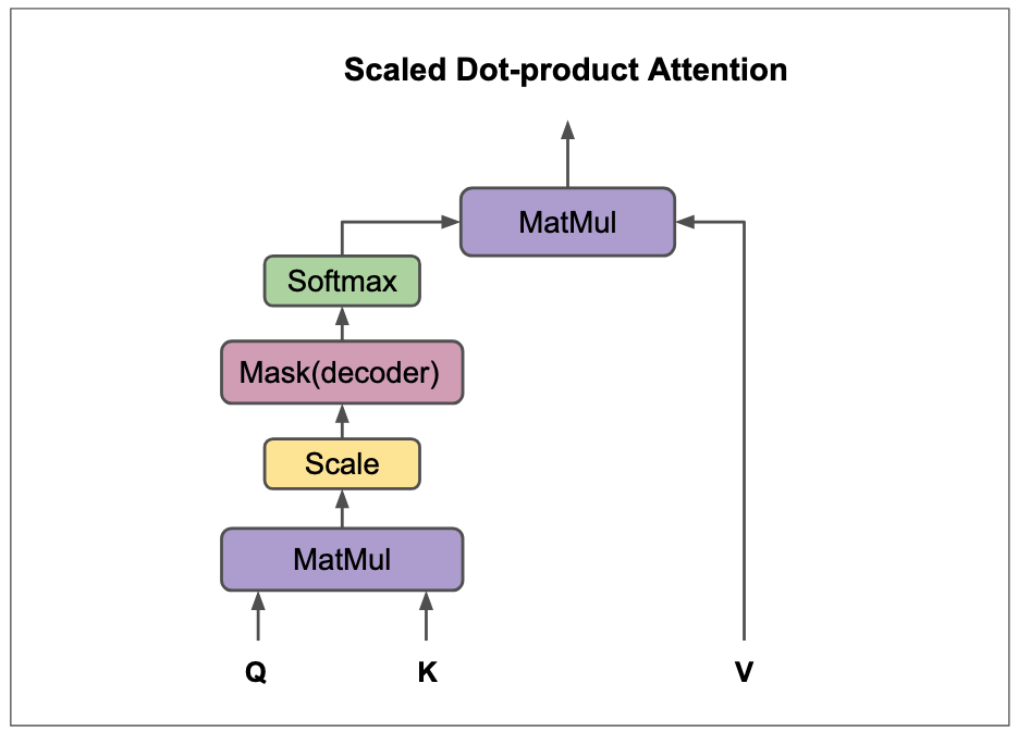
    return output, attention_weights

The attention weights are calculated by first calculating the dot product between the query and key vectors of each word in the sentence ( $Q * K^{T}$ ) . This dot product quantifies the similarity or relevance between each query word and each key word. Optionally, this value is often scaled by the square root of the dimension of the key vectors to improve the stability of the training (so-called Scaled Dot-Product Attention).

If a mask is present, the scores for certain connections are set to a negative value ( $- 1 e 9$ ). This large negative value ensures that the softmax function sets the corresponding weight in the attention matrix close to $0$ . The mask is used to prevent the model from accessing future words in the sequence. This is particularly important in decoder architectures or during training, where the model is supposed to generate words sequentially and may only use information from the previous words.

The Softmax Activationfunction function is then applied to the scores. This converts the similarity values into probabilities that sum to $1$ for each row. These probabilities are the actual attention weights, which indicate how strongly each word in the sentence influences the meaning of the current word.

Finally, the context vector for each word is generated by multiplying the attention weights by the value vectors. This context vector is a weighted sum of the value vectors of all words in the sentence and contains the relevant information of the entire sentence, taking into account the relationships between the words.

context_vectors, attention_matrix = calculate_attention(query, key, value)
 
print("Context vectors:", context_vectors)
print("Attention weights:", attention_matrix)

Context vectors: tensor([
    [0.3463, 0.3632, 0.5661, 0.5830, 0.5999, 0.5073, 0.6081, 0.6251, 0.6420, 0.6589],
    [0.6567, 0.6127, 0.6820, 0.6381, 0.5941, 0.6257, 0.4886, 0.4447, 0.4007, 0.3567],
    [0.5510, 0.5572, 0.6599, 0.6661, 0.6723, 0.6456, 0.4277, 0.4339, 0.4401, 0.4463],
    [0.3734, 0.4150, 0.6252, 0.6668, 0.7084, 0.4462, 0.5038, 0.5454, 0.5870, 0.6286],
    [0.6475, 0.5713, 0.6231, 0.5470, 0.4709, 0.6910, 0.6014, 0.5253, 0.4492, 0.3731],
    [0.4178, 0.3792, 0.6643, 0.6257, 0.5872, 0.4614, 0.6490, 0.6104, 0.5718, 0.5333]])
Attention weights: tensor([
    [0.3388, 0.0651, 0.1020, 0.1955, 0.1128, 0.1859],
    [0.0622, 0.3237, 0.2064, 0.1077, 0.1867, 0.1133],
    [0.0966, 0.2044, 0.3206, 0.1515, 0.1304, 0.0966],
    [0.1863, 0.1075, 0.1526, 0.3230, 0.0620, 0.1686],
    [0.1157, 0.2006, 0.1414, 0.0668, 0.3477, 0.1279],
    [0.1776, 0.1133, 0.0975, 0.1690, 0.1191, 0.3236]])

I will attempt to interpret the results. It is important to remember that this is a highly simplified, constructed example to illustrate the principle.

Attention weights

The attention weights, represented by the matrix, quantify the relevance of each individual word in the context of the entire sentence. Higher values indicate a stronger relationship between the query word (the row) and the key word (the column).

The diagonal of the matrix shows how strong the relationship of a word is to itself. Apart from that, the matrix shows the strength of the relationship between the query word and the other words in the sentence. Let’s look at the word May (first row): It has a comparatively strong relationship to itself ( $0.3388$ ) and a rather weak relationship to the word the ( $0.0651$ ). Interestingly, May also shows relatively high weights for be ( $0.1955$ ) and you ( $0.1859$ ). This could indicate that the model considers these words to be important for the context of May in the sentence “May the force be with you.”

For force (third row), we also see a strong self-relation ( $0.3206$ ), but also relatively strong relations to the ( $0.2044$ ) and be ( $0.1515$ ). This illustrates how the model recognizes semantic or syntactic relationships between words and weights them accordingly. The attention matrix allows us to analyze which words the model considers particularly relevant for the interpretation of a specific word in the sentence.

Context vector

The weighted sum of the value vectors forms the context vector. It captures the relevant information from the entire sentence, taking into account the relationships between the words. The attention weights determine how strongly the value vectors of the individual words contribute to the context vector. This creates a contextual representation of each word that is shaped by its relationships to other words in the sentence.

In the example, the context vector for May $[0.3463, ..., 0.6589]$ is strongly influenced by the value vectors of the words to which May assigns high attention weights (e.g., be and you, as observed above). The context vector for the, on the other hand, may be more strongly dominated by the value vectors of force and with, as these had high attention weights.

Importantly, we cannot directly read the specific influences of individual words from the numbers in the resulting context vector. We obtain this information from the previously calculated attention matrix. To better understand the quality of the context vectors and their relationship to the attention weights, we can again bring cosine similarity into play. It helps to check how similar the resulting context vectors are to each other and how this relates to the learned attention weights.

def cosine_similarity(vector1, vector2):
    return F.cosine_similarity(vector1.unsqueeze(0), vector2.unsqueeze(0)).item()
 
def compare_vectors(context_vectors, attention_matrix, word_list, word_index):
    """Compares the context vector of a word with the context vectors of the other words,
       taking into account the attention weights."""
 
    results = {}
 
    for other_word_index in range(len(context_vectors)):
        if word_index != other_word_index:
            similarity = cosine_similarity(
                context_vectors[word_index], 
                context_vectors[other_word_index])
            results[word_list[other_word_index]] = {
                "Similarity": similarity,
                "Attention weight": attention_matrix[word_index, other_word_index].item()
            }
    return results
 
# Input sentence
input_sentence = "May the force be with you"
word_list = input_sentence.split()
 
# Example call
results_may = compare_vectors(context_vectors, attention_matrix, word_list, 0)
results_the = compare_vectors(context_vectors, attention_matrix, word_list, 1)
 
# Output of results with tabbing
print(f"Comparison for 'May':")
print("  Word\t\tSimilarity\tAttention weight")
for word, data in results_may.items():
    print(f"  {word}\t\t{data['Similarity']:.4f}\t\t{data['Attention weight']:.4f}")
 
print(f"\nComparison for 'the':")
print("  Word\t\tSimilarity\tAttention weight")
for word, data in results_the.items():
    print(f"  {word}\t\t{data['Similarity']:.4f}\t\t{data['Attention weight']:.4f}")

Comparison for 'May':
  Word		Similarity	Attention weight
  the		0.9387		0.0651
  force		0.9561		0.1020
  be		0.9919		0.1955
  with		0.9491		0.1128
  you		0.9933		0.1859
 
Comparison for 'the':
  Word		Similarity	Attention weight
  May		0.9387		0.0622
  force		0.9944		0.2064
  be		0.9542		0.1077
  with		0.9913		0.1867
  you		0.9596		0.1133

The results of the script suggest a correlation between semantic similarity (measured by the cosine similarity of the context vectors) and the attention weights. Words that are considered by the model to be more relevant to the context of a particular query word (as indicated by high attention weights) also tend to have higher semantic similarity in their resulting context vectors. This is illustrated, for example, by comparing May with be and you (high similarity and high weights) versus May with the (lower similarity and lower weight).

Dynamic weighting through the attention mechanism enables the model to precisely understand the context of each word and extract relevant information for further processing. The resulting context vector thus serves as an enriched basis for subsequent layers in the Transformer model. To better understand this dynamic weighting, the question arises: Why do certain words in this matrix show a stronger relationship to each other than others? This is due to the weighting matrices ( $W_{Q}$ , $W_{K}$ , $W_{V}$ ) learned during training, which shape the relationships in the $Q$ , $K$ , and $V$ vectors in such a way that meaningful dependencies are recognized.

So far, we have examined how a single-head attention block works. We have seen how the input set is broken down into tokens and converted into Embeddings and similarity metrics. The query, key, and value matrices are derived from these input Embeddings and similarity metrics. These matrices are used to calculate attention weights, which are then used to weight the value matrices and generate contextualized vectors (context vectors).

At this point, a crucial aspect is missing in order to move from a single-head attention block to a multi-head attention block: the division into multiple “attention heads”. This is a central concept for further increasing the performance of transformers.

Multi-Head Attention: Multiple “Views” of the Context

So far, we have looked at the single-head attention mechanism, in which each word in the sentence focuses its attention on the other words and forms a single context vector. This is comparable to a person reading a text and trying to understand the meaning of each word in the overall context – but only from a single perspective. The multi-head attention mechanism is an ingenious extension of this concept. Imagine the same person reading the text, but now wearing $h$ different “glasses” or “perspectives.” Each pair of glasses (or “attention head”) allows them to recognize and focus on different aspects of the relationships between the words.

Why multiple heads?

The main reason for multi-head attention is that a single attention head may not be sufficient to fully capture the diverse relationships in a sentence. A word can simultaneously:

Have syntactic relationships to other words (e.g. subject-verb relationship: “The cat eats the mouse”).
Semantic relationships (e.g. synonyms, hypernyms: “river” and “stream” or “animal” as a superordinate term for “cat”).
Referential relationships (e.g. pronouns that refer to earlier nouns: “The boy played, he was happy.”).
Polysemy and multiple meanings: Words can have several meanings depending on context. For example, the word “bank” in English can refer to a financial institution (“I’m going to the bank”) or the side of a river (“He sat on the river bank”). Multi-head attention allows the model to focus on different contextual clues, helping it disambiguate which meaning is intended in a given sentence.

Each “head” can specialize in one of these aspects or learn a different type of attention, giving the model a more extensive and comprehensive understanding of the input text. It is as if several “experts” are looking at different aspects of the sentence at the same time and combining their findings.

The core idea

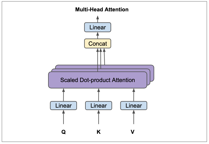
The input embeddings are not only projected once into query, key, and value matrices, but several times in parallel – separately for each head. Each of these projected sets of $Q$ , $K$ , $V$ is then passed through its own independent scaled dot product attention mechanism. The results of these $h$ independent attention calculations are then merged (concatenated) and transformed again to form the final output of the multi-head attention layer.

Visual analogy

I’ll try another analogy, another example.

Single-head: A single filter that analyzes an image and tries to find all features at once, which can result in an “average view.”
Multi-head: Several different filters working in parallel, each specializing in specific features. One filter looks for edges, another for colors, a third for textures, etc. The results of these specialized filters are then combined to obtain a more comprehensive understanding of the image.

Mathematical representation of multi-head attention

The formula for multi-head attention is as follows:

$MultiHead (Q, K, V) = Concat (head_{1}, \dots, head_{h}) W^{O}$

Where each individual $h e a d$ is calculated as follows:

$head_{i} = Attention (Q W_{Q}^{i}, K W_{K}^{i}, V W_{V}^{i})$

And the $Attention$ function (Scaled Dot-Product Attention) that we already know:

$Attention (Q, K, V) = softmax (\frac{Q ( K ) ^{T}}{d _{k}}) V$

Here, the following applies:

$Q, K, V$ : The original query, key, and value matrices derived from the input embeddings.
$W_{Q}^{i}, W_{K}^{i}, W_{V}^{i}$ : Projection matrices for the $i$ -th attention head. Each of these matrices has a dimension of $d_{m o d e l} \times d_{k}$ , where $d_{m o d e l}$ is the dimension of the input embeddings and $d_{k}$ is the dimension of the query/key vectors for one head. Often, $d_{k} = d_{m o d e l} / h$ .
$h$ : The number of attention heads.
$W^{O}$ : A final linear projection matrix that projects the concatenated outputs of the heads back to the original model dimension.

You can read more about the formulas in the paper. It gets exciting starting in chapter 3.2.1.

Steps in multi-head attention:

Linear projections for each head: For each of the $h$ attention heads, the input embeddings (or the output of the previous layer) are projected in parallel into separate query ( $Q_{i}$ ), key ( $K_{i}$ ), and value ( $V_{i}$ ) matrices. This is done by multiplying by the specific weight matrices $W_{Q}^{i}, W_{K}^{i}, W_{V}^{i}$ for each head. The key point here is that each head learns its own independent projections. This allows each head to focus on a different aspect of the input data.
Calculation of scaled dot-product attention: For each pair ( $Q_{i}, K_{i}, V_{i}$ ), the scaled dot-product attention is calculated separately. The result of each head is a set of contextualized vectors ( $head_{i}$ ).
Concatenation of head outputs: The $h$ outputs of the individual attention heads ( $head_{1}, \dots, head_{h}$ ) are placed side by side (concatenated), creating a single wider matrix.
Final linear projection: The concatenated matrix is then projected through another learned linear transformation matrix $W^{O}$ . This final transformation brings the output dimension back to the desired model dimension $d_{m o d e l}$ and allows the model to integrate the combined information from the different heads.

Practical example

It’s time for another practical example with code. To illustrate the concept of multi-head attention, we will build on our previous example. We will adapt the logic of the attention mechanism in a new function to show how multiple heads work in parallel and combine their results.

Assumptions for the example

Input embeddings: As before, we will continue to use $6 \cdot 10$ input embeddings for the sentence May the force be with you.
Number of heads ( $h$ ): I choose a small but understandable number, e.g., $h = 2$ heads.
Dimension per head ( $d_{k}$ ): If the dimension of the input embedding is $d_{m} = 10$ and we choose $h = 2$ , then the dimension per head is $d_{k} = d_{m} / h = 5$ . Each head will therefore work with 5-dimensional $Q$ , $K$ , $V$ vectors.
- This follows from the consideration that the total dimensionality of the outputs of the heads ( $h \cdot d_{k}$ ) should correspond to the original model dimension ( $d_{m}$ ) before the final projection is applied. This ensures that the dimension remains consistent throughout the entire Transformer block.
Weighting matrices: For the example, I will create simple, randomly initialized weighting matrices. In a real, trained model, these matrices would have been carefully learned to recognize specific linguistic patterns.

Then let’s get started.

1. Initializing the weighting matrices for each head

Each head needs its own projection matrices:

import matplotlib.pyplot as plt
import seaborn as sns
import pandas as pd
import torch
import torch.nn.functional as F
import numpy as np
torch.manual_seed(42)  # You can replace 42 with any integer of your choice
# Example embeddings (6 words, 10 dimensions)
word_embeddings = {
    "May": torch.tensor([0.1, 0.2, 0.3, 0.4, 0.5, 0.6, 0.7, 0.8, 0.9, 1.0]),
    
"the": torch.tensor([1.0, 0.9, 0.8, 0.7, 0.6, 0.5, 0.4, 0.3, 0.2, 0.1]),
    "force": torch.tensor([0.5, 0.6, 0.7, 0.8, 0.9, 1.0, 0.1, 0.2, 0.3, 0.4]),
    "be": torch.tensor([0.2, 0.4, 0.6, 0.8, 1.0, 0.1, 0.3, 0.5, 0.7, 0.9]),
    "with": torch.tensor([0.9, 0.7, 0.5, 0.3, 0.1, 1.0, 0.8, 0.6, 0.4, 0.2]),
    "you": torch.tensor([0.3, 0.1, 0.9, 0.7, 0.5, 0.2, 1.0, 0.8, 0.6, 0.4])
}
input_sentence_list = ["May", "the", "force", "be", "with", "you"]
input_embeddings = torch.stack([word_embeddings[word] for word in input_sentence_list])
d_model = input_embeddings.shape[1] # Dimension of input embeddings (here 10)
num_heads = 2                       # Number of attention heads
d_k = d_model // num_heads          # Dimension of the Q, K, V vectors per head (here 5)
W_Q = torch.randn(num_heads, d_model, d_k) # (heads, d_model, d_k)
W_K = torch.randn(num_heads, d_model, d_k)
W_V = torch.randn(num_heads, d_model, d_k)
W_O = torch.randn(d_model, d_model)        # Final projection matrix

2. Implementation of the multi-head attention logic

Next is the function that performs the steps of the multi-head attention mechanism described above.

def multi_head_attention(input_embeddings, W_Q, W_K, W_V, W_O, num_heads, d_k, mask=None):
    
# input_embeddings is expected here with batch dimension: (batch_size, seq_len, d_model)
    batch_size, seq_len, d_model = input_embeddings.shape
heads_output = []
attention_matrices = []
for i in range(num_heads):
# Project for the current head
        
# (batch_size, seq_len, d_model) @ (d_model, d_k) -> (batch_size, seq_len, d_k)
        Q_i = torch.matmul(input_embeddings, W_Q[i])
        K_i = torch.matmul(input_embeddings, W_K[i])
        
V_i = torch.matmul(input_embeddings, W_V[i])
# 2. Calculate scaled dot product attention for head_i
# scores: (batch_size, seq_len, seq_len)
scores = torch.matmul(Q_i, K_i.transpose(-2, -1)) / (d_k ** 0.5)
if mask is not None:
scores = scores.masked_fill(mask == 0, -1e9)
attention_weights_i = F.softmax(scores, dim=-1)
                
# head_i: (batch_size, seq_len, d_k)
        head_i = torch.matmul(attention_weights_i, V_i)
heads_output.append(head_i)
attention_matrices.append(attention_weights_i)
# 3. Concatenation of head outputs
    
# heads_output is a list of (batch_size, seq_len, d_k) tensors
    # concated_heads: (batch_size, seq_len, num_heads * d_k) = (batch_size, seq_len, d_model)
concated_heads = torch.cat(heads_output, dim=-1)
    
# 4. Final linear projection
    # output: (batch_size, seq_len, d_model) @ (d_model, d_model) -> (batch_size, seq_len, d_model)
output = torch.matmul(concated_heads, W_O)
return output, attention_matrices

# Call the multi-head attention function
input_embeddings_batched = input_embeddings.unsqueeze(0)
output_mha, attention_matrices_mha = multi_head_attention(
    input_embeddings_batched, W_Q, W_K, W_V, W_O, num_heads, d_k
)
print("\nOutput of the multi-head attention layer (context vectors):\n", output_mha.squeeze(0)) # squeeze(0) removes the batch dimension
print(f"\nNumber of attention matrices (corresponds to num_heads): {len(attention_matrices_mha)}")
print("\n--- Visualization of attention matrices ---")
plt.figure(figsize=(num_heads * 6, 6)) # Dynamically adjusts the figure size to the number of heads
for i, attn_matrix in enumerate(attention_matrices_mha):
    plt.subplot (1, num_heads, i + 1)
# CORRECTED: squeeze(0) to remove the batch dimension
df_attn = pd.DataFrame(attn_matrix.squeeze(0).detach().numpy(), index=input_sentence_list, columns=input_sentence_list)
        
sns.heatmap(df_attn, annot=True, cmap="YlGnBu", fmt=".2f", linewidths=.5, linecolor="gray")
    plt.title(f"Attention weights Head {i+1}")
    plt.xlabel("Keys (what is being paid attention to)")
    
plt.ylabel("Queries (which word is paid attention to)")
plt.tight_layout()
plt.show()

Output of the multi-head attention layer (context vectors):
 tensor([
    [-6.3872,  1.9858,  2.1712,  2.7969, -2.1122, -5.8285, -3.3943, -1.7054, -2.6450,  3.8029],
    [-6.0595,  2.2669,  2.7205,  3.5506, -2.4773, -6.7691, -3.6894, -2.3192, -2.7402,  5.1961],
    [-4.6440,  1.6299,  3.9077,  5.0117, -1.8828, -6.0060, -3.2956, -3.3168, -2.5437,  4.9490],
    [-5.7771,  2.0586,  2.5875,  3.0803, -1.6768, -5.7386, -3.5614, -2.2284, -2.6754,  4.2769],
    [-6.4755,  2.3926,  2.5579,  3.2462, -2.8572, -6.9736, -3.5434, -1.9716, -2.7969,  5.1418],
    [-6.8217,  3.0510,  3.1547,  2.3845, -1.8317, -6.1681, -2.8469, -1.6187, -2.7340,  4.0441]])
 
Number of attention matrices (corresponds to num_heads): 2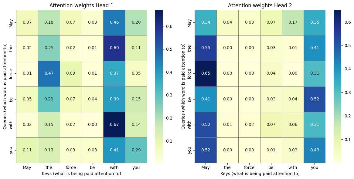

alt text

Interpretation of the results

Important note: As a reminder… The weight matrices $W_{Q}$ , $W_{K}$ , $W_{V}$ , and $W_{O}$ were initialized randomly and therefore do not reflect any meaningful linguistic or semantic meanings. However, a trained model would learn these matrices in such a way that they actually capture relevant dependencies. The purpose of this demonstration is to show the principle that each head can learn a different distribution of attention.

Attention Matrix Head 1

print(pd.DataFrame(attention_matrices_mha[0].squeeze(0).detach().numpy(), index=input_sentence_list, columns=input_sentence_list))

            May       the     force        be      with       you
May    0.068118  0.181340  0.071635  0.027055  0.456570  0.195282
the    0.015012  0.246116  0.019410  0.006160  0.599809  0.113493
force  0.007348  0.470308  0.094195  0.009372  0.368718  0.050059
be     0.054408  0.292597  0.065859  0.040474  0.393329  0.153334
with   0.018118  0.147041  0.020352  0.003969  0.671181  0.139338
you    0.106796  0.130137  0.028468  0.034135  0.407147  0.293317

Observations Head 1

In this matrix, there is a strong concentration of attention on the word with (column 5). Many words (May, the, be, with, you) direct a large part of their attention to with.
With itself in particular has the highest attention value ( $0.671$ ). In trained models, this is often the case for central elements in phrases or for words that play an important role in linking.
The column for the also shows comparatively higher attention values. Words such as force ( $0.470$ ) and be ( $0.292$ ) direct significant attention here.
Self-attention (diagonal): The values on the diagonal show how much attention a word pays to itself. with and the have relatively high values here, while May ( $0.068$ ) and force ( $0.009$ ), for example, draw less attention to themselves.
The word you (last row) distributes its attention relatively evenly among other words, with with still being the strongest focus ( $0.407$ ).

Possible hypothesis/interpretation Head 1

This head may specialize in capturing local dependencies and grammatical structures such as prepositional or noun phrases. The strong concentration on with and the could indicate that this head helps to identify phrases such as with you or the force as coherent units. It also seems to have a tendency to focus on functional words (such as articles or prepositions), which often play important syntactic roles.

Attention Matrix Head 2

print(pd.DataFrame(attention_matrices_mha[1].squeeze(0).detach().numpy(), index=input_sentence_list, columns=input_sentence_list))

            May       the     force        be      with       you
May    0.339671  0.036311  0.029780  0.072609  0.169864  0.351766
the    0.549202  0.000667  0.000758  0.028736  0.012748  0.407889
force  0.651215  0.000264  0.000342  0.038280  0.004499  0.305399
be     0.405897  0.003060  0.001443  0.031975  0.038848  0.518777
with   0.521837  0.008986  0.017760  0.074093  0.063290  0.314033
you    0.522649  0.000785  0.000491  0.012670  0.032367  0.431039

Observations Head 2

This head shows a very strong concentration of attention on the first word of the sentence, May (column 0). Almost all other words (the, force, be, with, you) focus most of their attention on May.
At the same time, there is also a clear focus on the last word, you (column 5). Many words look at both May and you.
The values in the middle columns (the, force, be, with) are mostly very low, which indicates less attention to these words when they serve as keys.
May and you also show a high level of self-attention.

Possible hypothesis/interpretation Head 2

This head may specialize in the endpoints of the sequence or in global relationships. The pattern suggests that it attempts to strongly associate the beginning of the sentence (May) and the end of the sentence (you) strongly, possibly to capture the overall context of a statement or to recognize relationships between parts of a sentence that are far apart. This is a typical feature of Transformer models, which, unlike RNNs, are able to model even far-reaching dependencies directly.

Summary of Multi-Head Attention

Comparing the two matrices reveals the core of the multi-head attention mechanism:

Head 1 seems to focus on local phrases and functional words (with, the). It is as if this head keeps an eye on the immediate grammar and relationships to direct neighbors.
Head 2, on the other hand, focuses on the beginning and end points of the sentence and largely ignores the details in the middle. This head could serve to capture higher-level structures or global dependencies across the entire length of the sentence.

Although these specific patterns arose randomly in our example, the diversity of attention patterns is precisely what makes the multi-head design so powerful. Each head learns (during training) to identify and weight a different type of relationship between words. Through the concatenation of the outputs and the final linear projection, these different perspectives are merged into a richer, multidimensional, and contextually enriched representation of each word in the sentence.

Conclusion and preview of Part 2

As we have now seen from the admittedly simple examples, the multi-head attention mechanism is much more than just a simple weighting of words. It enables the Transformer to capture different types of relationships and contexts in the data in parallel. Each head (in GPT-3, there are 96 heads, for example!) can focus on different semantic or syntactic aspects, resulting in a much richer and more nuanced representation of each word in the sentence. The ability to integrate these diverse perspectives is key to the performance of the Transformer architecture.

However, despite these attention mechanisms, the model still lacks crucial elements, which I will discuss in the second part in order to get a complete picture:

The attention mechanism itself is position-agnostic, meaning it knows nothing about the order of words. To remedy this, transformers integrate what is known as position encoding, which injects sequential information into the embeddings.
The contextualized information gained through attention must be further processed and transformed, which requires feed-forward networks.
Residual connections and layer normalization are essential for stable training of deep neural architectures, as they aid gradient flow and accelerate convergence.
Finally, all these components fit into the overall structure of the Transformer encoder and decoder, in which special masks play a critical role (e.g., the mask mentioned at the beginning that prevents “peeking” into future tokens).

In the next part, I will take a closer look at these topics and try to shed some light on them.

Digital garden

Explorer

The Transformer Architecture I