How can you teach a computer to recognize a number? Or characters? Cell phone numbers? Signs?

In this article, I will try to show you or give you a better understanding of how an artificial neural network works. Because the topic is very extensive, I wanted to incorporate a common thread. Using an example, the common thread, I will guide you through the topic. We will look at the Hello World! of machine learning: the MNIST dataset.

The MNIST dataset

The MNIST dataset is a well-known collection of handwritten digits that is of great importance for the development of algorithms for character recognition and image processing. In this chapter, I will examine the MNIST dataset in more detail and show how neural networks can be trained to recognize handwritten digits.

I will accompany all of this live with Python code.

At the end, I will show you a small Python application in which you can write digits with the mouse and read the classification made by the neural network. A quick note about the Python code. There is a much more elegant and efficient way to do this. However, I believe that the following code is easier for non-programmers or beginners to understand.

First, we’ll do a few imports. In Python, imports allow you to access existing code libraries instead of having to write everything from scratch. This saves time and allows me to use tried and tested functions.

import tensorflow as tf
from tensorflow.keras.models import Sequential
from tensorflow.keras.layers import Dense, Dropout
import matplotlib.pyplot as plt
import random
import numpy as np

Then we set a few seeds. Seeds are used in machine learning to control randomness in algorithms and achieve reproducible results. It is advisable to try different seeds to ensure the robustness of the model.

seed = 42
random.seed(seed)
np.random.seed(seed)
tf.random.set_seed(seed)

In Keras, the MNIST dataset, which consists of handwritten digits, is already stored. There is a load function in Keras that allows you to easily load this dataset into your model. I will make use of this here.

mnist = tf.keras.datasets.mnist
(x_train, y_train), (x_test, y_test) = mnist.load_data()

The following code block displays the first 20 images of the dataset.

fig = plt.figure(figsize=(12.5, 3))
for idx in np.arange(20):
  ax = fig.add_subplot(2, 10, idx + 1, xticks = [], yticks = [])
  ax.imshow(x_train[idx], cmap="gray")
  
ax.set_title(str(y_train[idx]))
fig.suptitle("20 of the digits in our dataset")
plt.show()

Overview of the MNIST dataset

The MNIST dataset consists of a total of $70.000$ images of handwritten digits. Of these, $60.000$ images are intended for training and $10.000$ images for testing. The images are black and white and have a size of $28 x 28$ pixels.

The dataset was created in the 1990s by Yann LeCun, Corinna Cortes, and Christopher J.C. Burges at the Courant Institute of Mathematical Sciences at New York University. It was developed to train and test algorithms for recognizing handwritten digits.

The handwritten digits in the dataset come from a variety of people and were written on standard forms. The digits are arranged in random order and have no special features or patterns that could influence recognition.

The dataset is a standard benchmark dataset and is often used to compare the performance of algorithms in the field of machine learning. The MNIST dataset is a simple and readily available dataset, which is why it is very often used in tutorials, training courses, and similar contexts. It is essentially the Hello World! of machine learning.

First, let’s take a closer look at a single image. To do this, we select one at random and plot it. On the one hand, the image as such, and on the other hand, how it is stored in memory and how computers use it, as numbers.

plt.rcParams.update({"font.size":8})
 
rnd = random.randint(0, len(x_train) - 1)
img = x_train[rnd]
ground_truth = y_train[rnd]
 
plt.figure(figsize = (20, 10))
plt.subplot(1,2,1)
plt.imshow(img, cmap="gray")
 
ax = plt.subplot(1,2,2)
ax.imshow(img, cmap="gray")
width, height = img.shape
thrs = img.max()/2.5
for x in range(width):
    for y in range(height):
        val = round(img[x][y], 2) if img[x][y] != 0 else 0
        ax.annotate(str(val), xy = (y, x),
                                horizontalalignment = "center",
                                verticalalignment = "center",
                                color = "white" if img[x][y] < thrs else "black")
 
print(f"Label of the randomly selected image: {ground_truth}")
plt.show()

Label of the randomly selected image: 4

The random image from the data set has the aforementioned $28 x 28$ pixels and is stored in grayscale. It is shown on the left as an image. The individual gray scale values, the numbers representing each pixel, are shown in the output on the right. These are originally values between $0$ and $255$ , or $8$ bits per pixel. The value indicates how bright this pixel is.

These numerical values are the ones that are fed into the input layer, which will be described later.

Feature maps

While the above image from the MNIST dataset has one feature map, the grayscale values, the situation is different for color images. Color images have a separate feature map for each color channel: red, green, blue. 8 bits per channel are commonly used, which results in a total of $(2^{8})^{3} = 2^{24} = 16.777.216$ possible colors. When recognizing digits, we can of course do without the color channels. Gray levels are sufficient.

The three feature maps of an RGB image.

The neural network

Back to our example: We have $28 * 28 = 784$ pixels, each with a value. And these $784$ pixels need to be analyzed. Our brain has learned to link these pixels in such a way that we can easily recognize the number. We still have to teach this to the neural network.

So we take these $784$ pixels as input for our neural network. The task specifies that we need $10$ outputs, the digits $0$ to $9$ . We refer to the inputs as the input layer, and the outputs as the output layer. Everything in between is called the hidden layer(s). It is already clear at this point that our trained neural network can only be used for this task.

For easier handling, we transform the input matrix of $28 * 28$ pixels into a tensor of size $784$ . We then have $784$ pixels or inputs arranged in a row, which in turn are connected to each neuron in the following layer. Each of these neurons is in turn connected to every neuron in the following layer, right up to the output layer. This architecture is known as a multilayer perceptron. There are other architectures where this is not the case, but more on that later.

Feedforward network or multilayer perceptron. Image source

The term neuron has been used so frequently that we should take a closer look at it.

The neuron

The neuron is a simple artificial neural network (ANN) that was developed in the early days of artificial intelligence (AI). It is a fundamental concept in machine learning and is often used as an introduction to the topic of deep neural networks (DNNs).

A neuron with input vector, bias, activation function, and output. Image source

A neuron consists of an input vector $a_{i}$ , a weight vector $w_{i}$ , an offset or bias $b$ , and an activation function $σ$ . Each input value is assigned a weight, which determines the influence of the respective value on the output of the neuron. The sum of all weighted input values is then passed through the activation function, which decides whether and how the neuron “activated” or not. A look at different activation functions is also included in this article. You can find a brief overview in this image. The x-axis represents the value that flows into the activation function and the y-axis represents the corresponding activation.

Three of the most common activation functions: sigmoid, tanh, and ReLU.

The neuron can be trained for a variety of tasks, including classification and regression. In the case of classification, the neuron is trained to classify an input into one of several predefined categories. In the case of regression, the neuron is trained to predict a continuous output based on an input.

Training a neuron essentially consists of adjusting the weights to improve the prediction accuracy of the model. This is done using an optimization algorithm such as the gradient descent method, which updates the weights during so-called backpropagation based on the errors made by the neuron in its prediction.

So we have $784$ of these neurons in the input layer and $10$ in the output layer, since we want to predict the digits $0...9$ . For better results or faster training, the values of the inputs are scaled. Non-universal reasons for this are:

Better convergence: Scaling the inputs to a similar value range can improve the convergence of the training process. If the inputs have widely varying value ranges, this can cause some weights in the network to be updated faster than others. This can lead to slower convergence or even training getting stuck. Scaling the inputs can reduce these problems.
Avoiding numerical instability: Neural networks often perform mathematical operations such as calculating activation functions or updating weights. If the inputs have large values, these operations can lead to numerical instability, for example through overflow or underflow. Scaling the inputs to a smaller value range can avoid such problems.
Better interpretability: Scaled inputs can also lead to better interpretability of the results. If the inputs are scaled to a specific value range, the weights in the network can be directly related to the meaning of the input variables. This can help to better understand the impact of the inputs on the model’s predictions.

The input vector then looks like this:

print(f"Shape of x_train before reshaping: {x_train.shape}\n"
      f"Maximum value of an entry: {x_train[rnd].max()}\n"
      f"Shape of a single image/input vector: {x_train[rnd].shape}")
 
x_train = x_train.reshape((-1, 28 * 28)).astype("float32") / 255
x_test = x_test.reshape((-1, 28 * 28)).astype("float32") / 255
 
print(f"Shape of the data after reshaping: {x_train.shape}\n"
      f"Maximum value of an entry: {x_train[rnd].max()}\n")

Shape of x_train before reshaping: (60000, 28, 28)
Maximum value of an entry: 255
Shape of a single image/input vector: (28, 28)
Shape of the data after reshaping: (60000, 784)
Maximum value of an entry: 1.0

One-hot encoding

Next, I perform one-hot encoding. One-hot encoding is a technique for representing categories as binary vectors. Each category is assigned a vector, where one position represents the category and all other positions contain zeros. This encoding is often used in machine learning modeling. In the case of our handwritten digits, each digit would be assigned a unique category. For example, a $0$ could be encoded as $[1, 0, 0, 0, 0, 0, 0, 0, 0, 0]$ , while a $1$ would be encoded as $[0, 1, 0, 0, 0, 0, 0, 0, 0, 0]$ , etc.

Especially for classification problems (such as here with the MNIST dataset) the output variables should be converted into a suitable form so that they can be used in the model. By using one-hot encoding, the output variables can be used more efficiently with the model, as they can be represented as numerical values. This facilitates the calculations and training of the model.

y_train = tf.keras.utils.to_categorical(y_train)
y_test = tf.keras.utils.to_categorical(y_test)
print(f"One-hot encoded label: \n{y_train[rnd]}\n"
      f"Ground Truth / Label: {ground_truth}")

One-hot encoded label: 
[0. 0. 0. 0. 0. 0. 0. 0. 0. 1.]
Ground Truth / Label: 4

Building the neural network

Now let’s move on to the actual neural network. Let’s start with the implementation.

First, we define a so-called early stopping callback. Early stopping is a method in machine learning where the training of a model is terminated prematurely to avoid overfitting, based on the observation of validation errors during each epoch.

callback = tf.keras.callbacks.EarlyStopping(
    monitor="val_accuracy",
    patience=10
)

Next comes the model. I am using a sequential model here. A sequential model in TensorFlow is a linear stack of layers or (hidden) layers that are executed one after the other. It enables the construction and training of neural networks for various machine learning tasks by using different layer types.

Let’s define the sizes of the individual layers. We specify the number of desired neurons.

input_layer_size = 28 * 28
first_layer_size = 256
second_layer_size = 128
output_layer_size = 10

model = tf.keras.Sequential([
    tf.keras.layers.Dense(first_layer_size, activation="relu", input_shape=(input_layer_size,)), 
    tf.keras.layers.Dense(second_layer_size, activation="relu"),
    tf.keras.layers.Dense(output_layer_size, activation="softmax")
])

The above code defines a TensorFlow Keras sequential model with three dense layers. The first layer has first_layer_size neurons and a ReLU activation, the second has second_layer_size neurons and a ReLU activation, and the last has output_layer_size neurons and a softmax activation.

The model must then be compiled. Here, you can pass on a wide variety of parameters. I will limit myself here (in the code below) to the optimizer, the loss, and the metrics. A brief description:

Optimizer: An optimizer is an algorithm that adjusts the weights of a neural network to minimize error.
Loss: The loss is a function that measures the error between the model’s predictions and the actual values. I am using categorical_crossentropy, which is a loss function used in multi-class classification tasks, measuring the difference between predicted and true probability distributions.
Metrics: Metrics are benchmarks used to evaluate the performance of a model, e.g., accuracy or F1 score.

Usually, a learning rate is also passed, which is used to adjust the weights during backpropagation. The Adam optimizer used makes this step unnecessary.

The Adam optimizer is an optimization algorithm that uses an adaptive learning rate. Unlike other optimizers such as gradient descent, which require a fixed learning rate to be specified, the Adam optimizer automatically adjusts the learning rate to the data. It calculates and updates the learning rate based on the moments of the gradients. This eliminates the need to pass a fixed learning rate to the Adam optimizer.

I have written a more detailed description later in this post.

model.compile(
    optimizer="Adam",
    loss="categorical_crossentropy",
    metrics=["accuracy"]
)

Now let’s output some information about our neural network.

print(model.summary())

Model: "sequential"
    
_________________________________________________________________
Layer (type)                Output Shape              Param #  
 
=================================================================
dense (Dense)               (None, 256)               200960
dense_1 (Dense)             (None, 128)               32896
                                                                               
dense_2 (Dense)             (None, 10)                1290      
                                                                  
=================================================================
Total params: 235,146
Trainable params: 235,146
Non-trainable params: 0
_________________________________________________________________
None

So we have around $200.000$ parameters that need to be adjusted during training. This is by no means a particularly large network, which can often have parameters in the $9$ -digit range, but it is still too many to adjust the network (multiple times) by hand and it is hopefully enough parameters to be able to recognize the digits.

history = model.fit(
    x_train, 
    y_train, 
    epochs=50, 
    batch_size=128, 
    callbacks=[callback], 
    validation_split=0.2, 
    verbose=0
)

In the above step, the training is now carried out. Here, too, several parameters are passed:

Epochs: An epoch is an iteration over the entire training dataset during the training process of a model. By running through multiple epochs, the model can access the entire training dataset several times and adjust its weights accordingly to achieve better performance.
Batch Size: The batch size specifies how many training examples are processed simultaneously in one step. The batch size affects how many training examples are processed at once. A larger batch size can speed up training, while a smaller batch size can allow for more accurate updating of the weights.
Validation Split: During training, the validation-training split is used to monitor the progress of the model and avoid overfitting. A portion of the training data is separated as validation data and used separately to evaluate the model’s performance on unknown data and adjust hyperparameters.

fig, (ax1, ax2) = plt.subplots(2, 1, figsize=(8, 6))
 
# Plot 1
ax1.plot(history.history["accuracy"])
ax1.plot(history.history["val_accuracy"])
ax1.set_title("model accuracy")
ax1.set_ylabel("accuracy")
ax1.set_xlabel("epoch")
ax1.legend(["train", "test"], loc="upper left")
 
# Plot 2
ax2.plot(history.history["loss"])
ax2.plot(history.history["val_loss"])
ax2.set_title("model loss")
ax2.set_ylabel("loss")
ax2.set_xlabel("epoch")
ax2.legend(["train", "test"], loc="upper left")
 
plt.tight_layout()
plt.show()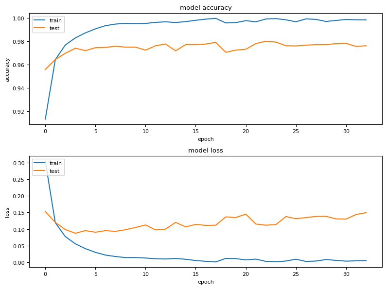

The plot above shows the accuracy and loss of training and validation after each epoch. These curves show the general performance. However, more specific information can also be derived. For example, if the accuracy of the training is very good, but that of the validation is not, the model is probably overfitted. If both accuracies are poor, it is underfitted. More on this shortly. You too can see, that the ealy-stopping callback stopped the training process early, since we planned with 50 epochs.

If we believe that the training of our network was sufficient, we can test its performance on previously unseen material.

# Evaluation of the model
test_loss, test_acc = model.evaluate(x_test, y_test)
print("Test accuracy:", test_acc)

313/313 [==============================] - 1s 3ms/step - loss: 0.1239 - accuracy: 0.9786
Test accuracy: 0.978600025177002

With the above neural network, we achieve an accuracy of $97.8%$ . For comparison, the best models achieve accuracies of over $99.8%$ .

A slightly different comparison to narrow it down. Assuming that the digits were evenly distributed in the data set and each digit had a probability of $10%$ , and my model would say that each digit is not the $5$ , then the model would be correct in $90%$ of cases. Of course, this comparison is a little flawed.

Now, the above model may have an overfitting problem because it achieves almost $100%$ accuracy during training but cannot maintain that accuracy in validation. Therefore, I am now trying to improve the result by using a so-called dropout layer.

Underfitting, overfitting, and dropout

Underfitting and overfitting are problems that can occur when training machine learning models. Underfitting occurs when the model is unable to capture the training data well, while overfitting occurs when the model is too closely adapted to the training data and does not generalize well to new data.

Dropout in different hidden layers. Image source

There are various techniques for preventing overfitting. One of these is called dropout.

During training, neurons are randomly deactivated by setting their outputs or weights to zero. This reduces redundancy and makes the model more robust. Dropout helps to improve the generalization ability of the model and improves performance on new data.

It is implemented quite quickly. I can simply add a layer to the sequential model and recompile it. I tell the layer to drop $20%$ of the neurons. This happens randomly during each training run.

Then we restart training with the modified model. The steps are like before, we just added the dropout layer.

model2 = tf.keras.Sequential([
    tf.keras.layers.Dense(first_layer_size, activation="relu", input_shape=(input_layer_size,)),
    tf.keras.layers.Dropout(0.2),
    tf.keras.layers.Dense(second_layer_size, activation="relu"),
    tf.keras.layers.Dense(output_layer_size, activation="softmax")
])

model2.compile(
    optimizer="Adam",
    loss="categorical_crossentropy",
    metrics=["accuracy"]
)

print(model2.summary())

Model: "sequential_1"
_________________________________________________________________
Layer (type)                Output Shape              Param #   
=================================================================
dense_3 (Dense)             (None, 256)               200960
                                                          
dropout (Dropout)           (None, 256)               0         
                                                
dense_4 (Dense)             (None, 128)               32896     
                                                
dense_5 (Dense)             (None, 10)                1290
                                                            
=================================================================
Total params: 235,146
Trainable params: 235,146
Non-trainable params: 0
_________________________________________________________________
None

# Training the model
history = model2.fit(
    x_train, 
    y_train,
    epochs=50, 
    batch_size=128, 
    callbacks=[callback], 
    validation_split=0.2, 
    verbose=0
)

fig, (ax1, ax2) = plt.subplots(2, 1, figsize=(8, 6))
 
# Plot 1
ax1.plot(history.history["accuracy"])
ax1.plot(history.history["val_accuracy"])
ax1.set_title("model accuracy")
ax1.set_ylabel("accuracy")
ax1.set_xlabel("epoch")
ax1.legend(["train", "test"], loc="upper left")
 
# Plot 2
ax2.plot(history.history["loss"])
ax2.plot(history.history["val_loss"])
ax2.set_title("model loss")
ax2.set_ylabel("loss")
ax2.set_xlabel("epoch")
ax2.legend(["train", "test"], loc="upper left")
 
plt.tight_layout()
plt.show()

test_loss, test_acc = model2.evaluate(x_test, y_test)
print("Test accuracy:", test_acc)

313/313 [==============================] - 1s 3ms/step - loss: 0.0870 - accuracy: 0.9811
Test accuracy: 0.9811000227928162

Compared to our previous result ( $97.8%$ ), we have achieved a small improvement: $98.1%$ . I can make this comparison here because I set the seeds used to generate the pseudo-random numbers at the beginning. This is to ensure that everything related to randomization is reproducible.

Next, we look at the error matrix to see where the model could make even better predictions or where it may still have difficulties.

Confusion matrix

The error matrix (also known as the confusion matrix) is a table that shows the performance of a classification model. It shows the number of correctly and incorrectly classified examples for each class.

The confusion matrix consists of four main components:

true positives (TP)
true negatives (TN)
false positives (FP)
false negatives (FN).

TP are the correctly classified positive examples, TN are the correctly classified negative examples, FP are the examples incorrectly classified as positive, and FN are the examples incorrectly classified as negative.

The confusion matrix allows us to derive various performance metrics, such as accuracy, precision, recall, and F1 score. It also gives us insights into the types of errors the model makes and can help us improve the model’s performance by analyzing the errors and making appropriate adjustments.

The confusion matrix is an important tool in the evaluation of classification models and helps us understand and interpret the strengths and weaknesses of the model.

I would like to use it here to estimate where the model makes incorrect predictions. To do this, we first need to let the model make the predictions.

y_pred = model2.predict(x_test)
 
print(
    f"y_pred shape: {y_pred.shape}\n"
    f"y_test shape: {y_test.shape}"
)

313/313 [==============================] - 1s 2ms/step
y_pred shape: (10000, 10)
y_test shape: (10000, 10)

The data is still one-hot encoded, which we can see from the second dimension of the shape. This means we cannot yet create an error matrix. Let’s recall what one of the $10000$ arrays looks like.

print(
    f"Array: {y_pred[1]}\n"
    f"Max. value: {np.max(y_pred[1])}\n"
    f"Position of max. value: {np.argmax(y_pred[1])}"
)

Array: [3.5470648e-16 1.0974492e-12 1.0000000e+00 9.9223222e-14 1.7690568e-29 1.0701757e-20 3.9431806e-20 9.0893782e-17 3.4036694e-14 6.1461460e-25]
Max. value: 1.0
Position of max. value: 2

The array contains the probability of each of the $10$ predictable digits being the correct digit.

In the above example, the model is very confident. The highest probability is given as $1$ . The network is therefore over $100%$ certain that this is the correct digit. And this probability is in the second position in the array, representing $3$ .

I now apply this procedure to all data.

y_pred = np.argmax(y_pred, axis = 1)
y_test = np.argmax(y_test, axis = 1)

Now the data is in the correct format and I can create the error matrix.

from sklearn.metrics import confusion_matrix
 
cm = confusion_matrix(y_test, y_pred)
 
labels = np.arange(10)
 
plt.imshow(cm, interpolation="nearest", cmap=plt.cm.Blues)
plt.title("Confusion Matrix - MNIST")
plt.colorbar()
tick_marks = np.arange(len(labels))
plt.xticks(tick_marks, labels)
plt.yticks(tick_marks, labels)
plt.xlabel("Predicted Class")
plt.ylabel("Actual Class")
 
 
thresh = cm.max() / 2.
for i in range(cm.shape[0]):
    for j in range(cm.shape[1]):
        plt.text(j, i, format(cm[i, j], "d"),
                 horizontalalignment="center",
                 color="white" if cm[i, j] > thresh else "black")
plt.tight_layout()
plt.show()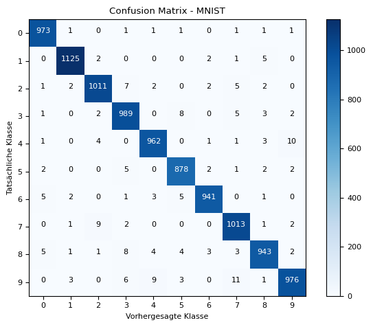

What we can see from this graph… The correct digit is plotted on the y-axis, and the predicted digit on the x-axis. If these values match, the counter is incremented (on the diagonal). The higher the values on the diagonal, the better, because the model has predicted more correctly.

The fields around it indicate how often the network mistook, for example, a $2$ for a $5$ , which occurred $1$ time here. Compared to the other incorrectly predicted digits, the $10$ incorrect predictions for the $4$ , which was mistaken for a $9$ by the neural network, seem particularly high. This seems plausible to me, as these digits often look very similar, at least when I write them.

In this way, it is possible to verify the plausibility of the neural network’s predictions to a certain extent.

So now I have shown how to program the neural network. But what happens during training is the really exciting part. Let’s move on to training.

Training the neural network

The neural network learns by adjusting its weights and bias values to improve its predictions. It repeats this over and over again until the accuracy is sufficient or the training has to be stopped because the model may not be complex enough. Training a neural network traditionally follows these steps.

Initialization: The weights and bias values of the network are initialized randomly, often with a small normal distribution to promote more efficient convergence.
Forward propagation: The input data is passed through the network, using the activation functions and weights to calculate the network’s output. Each layer of the network performs a linear transformation of the inputs and then applies a nonlinear activation function such as the sigmoid, ReLU, or tanh function.
Error calculation: The difference between the calculated output of the network and the actual output values is calculated using an error or cost function such as the mean squared error (MSE) for regressions or the cross-entropy error for classification. This function measures the performance of the network and serves as the basis for adjusting the weights.
Backpropagation: The error is propagated backward through the network to calculate the gradient of the error function with respect to the weights and bias values. This is achieved using the chain rule of differentiation by tracing the error back from the output layer to the input layer. The gradient indicates how much the weights and bias values need to change to reduce the error.
Weight update: An optimizer, such as gradient descent or its variants such as SGD, Adam, or RMSprop, is used to update the weights and bias values based on the calculated gradient. The learning rate, which determines the size of the update steps, can be adjusted to control convergence and avoid overfitting.
Repetition: Steps 2-5 are repeated for a certain number of epochs or until a termination criterion is met. Typical termination criteria include reaching a certain level of accuracy on a validation dataset or the absence of significant improvement in performance over several epochs.

The interaction of backpropagation, gradient descent, and optimizers is intended to find the global minimum of the cost function. Image source

In the following, I will first discuss a few of the cost functions. Then I will describe forward and backward propagation as well as the gradient descent method in more detail. Finally, I will attempt to provide a (numerical) example. Another post will then deal with optimizers.

Forward propagation

Forward propagation is the process by which input data flows through the neural network to generate a prediction. In each layer, the inputs are multiplied by the weights and the biases are added. The resulting sum is then passed through an activation function such as the sigmoid function or the ReLU function to calculate the activations of the neurons. This process is repeated for each layer until the output is reached. Mathematically expressed:

$z^{(l)} = W^{(l)} \cdot a^{(l - 1)} + b^{(l)}$

$a^{(l)} = f (z^{(l)})$

Here, $z^{(l)}$ is the weighted sum of the inputs in layer $l$ , $W^{(l)}$ are the weights, $a^{(l - 1)}$ are the activations of the previous layer, $b^{(l)}$ are the biases, and $f ()$ is the activation function.

Error calculation: Cost functions

In this section, I would like to mention a few of the most common cost functions.

Mean Squared Error (MSE): The MSE function measures the average squared error between the actual and expected outputs. It is often used in regression problems where the goal is to estimate a continuous output. The function calculates the squared difference between each actual and expected output and then takes the average across all examples. The MSE function is sensitive to outliers because the squared error increases sharply as the difference between the actual and expected values increases.

$MSE = \frac{1}{n} \sum_{i = 1}^{n} (y_{i} - \overset{y}{^}_{i})^{2}$

Mean Absolute Error (MAE): The MAE function measures the average absolute error between actual and expected outputs. Unlike the MSE function, which considers the squared error, MAE considers the absolute error. This means that outliers in the data have less influence on the cost than when using MSE. The MAE function is also useful for regression problems and is often used when it is important to understand the average error in the actual units of output.

$M A E = \frac{1}{n} \sum_{i = 1}^{n} ∣ y_{i} - \overset{y}{^}_{i} ∣$

Binary Cross-Entropy: This function is used when dealing with a binary classification problem where the output is either 0 or 1. The function measures the error between the actual and expected outputs, where the outputs are interpreted as probabilities. It uses the logarithmic function to calculate the error, with a higher error occurring when the actual output deviates significantly from the expected output. The binary cross-entropy function is often combined with the sigmoid activation function in the output layer.

$B ina ry C ross E n t ro p y = - \frac{1}{n} \sum_{i = 1}^{n} [y_{i} lo g (\overset{y}{^}_{i}) + (1 - y_{i}) lo g (1 - \overset{y}{^}_{i})]$

Categorical Cross-Entropy: This function is used when dealing with a multi-class classification problem where the output is divided into several classes. Similar to the binary cross-entropy function, it measures the error between the actual and expected outputs, where the outputs are interpreted as probabilities. The categorical cross-entropy function uses the logarithmic function to calculate the error, where a higher error occurs when the actual output deviates significantly from the expected output. It is often combined with the Softmax Activationfunction activation function in the output layer to normalize the probabilities for each class.

C a t e g or i c a lC ross E n t ro p y = - \frac{1}{n} i = 1 \sum n j = 1 \sum m y_{ij} lo g (\overset{y}{^}_{ij})

In the equations, $y$ and $\overset{y}{^}_{i}$ represent the actual (ground truth) and predicted values or outputs of the model, respectively.

In the context of regression (as with MSE and MAE), $y$ represents the actual value of the target variable (actual prices in a price prediction model) and $\overset{y}{^}_{i}$ represents the values predicted by the model.
In binary cross entropy loss, $y$ represents the actual class (either $0$ or $1$ ) and $\overset{y}{^}_{i}$ represents the probability that the model predicts this class.
In categorical cross entropy, $y_{ij}$ represents the probability that the model predicts example $i$ as class $j$ , while $y_{ij}$ is the actual probability that example $i$ is class $j$ . In all cases, $y$ is the ground truth value and $\overset{y}{^}_{i}$ is the model prediction.

Backpropagation

Backward propagation is the process of passing the error backward through the network to calculate the gradient of the error function with respect to the weights and biases. The gradient is calculated using the chain rule of differentiation and propagated from the output layer to the input layer. Mathematically expressed:

$δ^{(L)} = \nabla_{a} E ⊙ f^{'} (z^{(L)})$

$δ^{(l)} = ((W^{(l + 1)})^{T} \cdot δ^{(l + 1)}) ⊙ f^{'} (z^{(l)})$

Here, $δ^{(L)}$ is the error in layer $l$ , $\nabla_{a} E$ is the gradient of the error function with respect to the outputs, $f^{'} (\cdot)$ is the derivative of the activation function, $z^{(L)}$ is the weighted sum of the inputs in layer $l$ , and $⊙$ stands for element-wise multiplication.

Weight update

Weight update is a crucial step in training neural networks. After the gradient of the error function has been calculated, the weights and biases are updated based on this gradient and a learning rate $α$ . This is done to gradually minimize the error and adjust the model. Weight updating is performed by applying the gradient descent method:

The change in weights $Δ W^{(l)}$ and biases $Δ b^{(l)}$ is calculated by multiplying the negative gradient by the learning rate.
The weights and biases are updated according to the calculated change.
This process is repeated iteratively to minimize the error over several epochs and improve the model.

The learning rate influences the size of the update steps and is crucial for the convergence of the model. A learning rate that is too high can lead to unstable or divergent solutions, while a learning rate that is too low can lead to slow convergence or local minima. Therefore, selecting a suitable learning rate is crucial for training a neural network.

In a separate post, I will use an example to show how the interaction works.

Summary

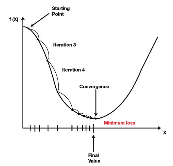
Gradient descent method in 3-dimensional space. Image source

The goal of the method described above, which combines backpropagation, mean squared error (MSE)(for example), and stochastic gradient descent (SGD), is to train a neural network to find a global minimum of the cost function in a high-dimensional space. By gradually adjusting the weights and bias values using the gradient descent method, the cost function is continuously minimized to achieve optimal network performance for the given task. This process enables the network to learn complex patterns and relationships in the data and make accurate predictions.

Activation Functions

Activation functions are also an important part of any artificial neural network. They determine how the network responds to certain inputs and contribute significantly to the performance and accuracy of an ANN. In this section, we will learn about some of the most commonly used activation functions in ANNs.

Sigmoid function

The sigmoid function is often used in binary classification problems. The function uses an S-shaped curve that allows for a smooth overlap between classes. It returns an output value between 0 and 1. One disadvantage of the sigmoid function is that it is susceptible (I learned a new word here ;)) to the problem of gradient vanishing when the weights become too large.

Sigmoid gradient vanishing describes the phenomenon of individual gradients approaching zero. This is because the derivative of the sigmoid function becomes very small for very large or very small inputs. If the gradient is close to zero, the ANN may train very slowly or stop training altogether, because the gradient is needed to update the parameters of the ANN. Solutions can include other activation functions, for example ReLU, or the use of methods such as gradient clipping or batch normalization.

A common use case for sigmoid activation functions is in binary classification problems, where the model must make predictions that are either true or false (Is there a dog in the picture?). The formula for the sigmoid activation function is:

$f (x) = \frac{1}{1 + e ^{- x}}$

The activation function and derivative are shown here.

Sigmoid activation function with derivative.

Rectified Linear Unit (ReLU)

The ReLU function (Rectified Linear Unit) is a linear function that returns zero for negative inputs and the input value itself for positive inputs. This makes the ReLU function particularly useful when learning non-linear functions. However, one disadvantage of the ReLU function is that it is susceptible to the dead neuron effect, whereby neurons that produce a negative output are set to zero and can no longer be trained.

The Dying ReLU problem describes the effect when a neuron in the ANN no longer outputs activation due to the activation function used and remains inactive for all subsequent layers of the neural network. This limitation can cause the ANN to malfunction and impair performance. Solutions to this problem include the Leaky or Parametric ReLU activation function. These ensure that the neuron outputs a small activation for negative inputs. Alternatively, the ANN can be initialized so that the weights do not become too negative.

The ReLU activation function is a common choice for deep learning problems that involve approximating functions that exhibit nonlinear relationships. An example could be predicting the sale price of a house based on various characteristics such as size, location, and age.

The formula for the ReLU activation function is:

$f (x) = ma x (0, x)$

The ReLU function itself and its derivative can be represented graphically as follows:

ReLU activation function with derivative.

Tanh (hyperbolic tangent)

The tanh function describes an S-shaped curve similar to the sigmoid function. However, it returns output values between -1 and 1, which makes it more suitable for problems where negative outputs are possible. One disadvantage of the Tanh function, however, is that it is also susceptible to the vanishing gradient problem.

A common use case for the hyperbolic tangent activation function is in deep learning problems that involve approximating functions more complex than the ReLU function. An example could be predicting the movement of an object based on its velocity and acceleration.

The formula for the hyperbolic tangent activation function is:

$f (x) = t anh (x)$

The hyperbolic tangent function and its derivative in a graph: 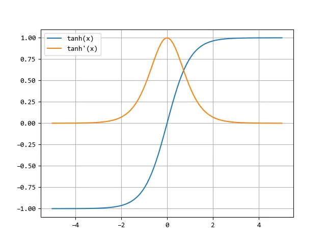Tanh activation function with derivative. Image by author

There are other activation functions used in artificial neural networks, but the ones mentioned above are some of the most common. Choosing the right activation function depends on the type of problem and the requirements of the model. It is important to take the time to understand and compare the different activation functions in order to achieve the best possible performance for your problem.

Optimizers

In this section, I would like to briefly describe a few of the most common optimizers: Stochastic Gradient Descent (SGD), Adam (Adaptive Moment Estimation), and RMSProp (Root Mean Squared Propagation). I plan to discuss a few optimizers in more detail in a separate post.

Stochastic Gradient Descent (SGD):

SGD is one of the most basic optimizers for training neural networks. It is based on the gradient descent method, in which the weights are updated after each mini-batch of training data to minimize the error. The weights are updated along the direction of the negative gradient of the error function, thereby improving the model step by step.

$W^{(t + 1)} = W^{(t)} - α \cdot \nabla E (W^{(t)})$

where $α$ is the learning rate and $\nabla E (W^{(t)})$ is the gradient of the error function $E$ with respect to the weights $W$ .

Adam (Adaptive Moment Estimation)

Adam is a popular optimizer that combines the advantages of AdaGrad and RMSProp. It uses both an adaptive learning rate approach and momentum estimation to adjust the weights during training. Adam adjusts the learning rate for each weight based on past gradients and squares of the gradients, making it effective and robust and frequently used in practice.

$m^{(t + 1)} = β_{1} \cdot m^{(t)} + (1 - β_{1}) \cdot \nabla E (W^{(t)})$

$v^{(t + 1)} = β_{2} \cdot v^{(t)} + (1 - β_{2}) \cdot (\nabla E (W^{(t)}))^{2}$

$W^{(t + 1)} = W^{(t)} - \frac{α}{v ^{(t + 1)} + ϵ} \cdot m^{(t + 2)}$

where $m^{(t)}$ and $v^{(t)}$ are the moving averages of the gradient and its squares, $β_{1}$ and $β_{2}$ are the exponential factors, $α$ is the learning rate, and $ϵ$ is a value used for stabilization.

RMSProp (Root Mean Square Propagation)

RMSProp is a variant of the gradient descent method in which the learning rate for each weight is adjusted based on the average quadratic gradient for that weight. This allows the learning rate to be adjusted individually for each weight, which is particularly helpful when gradients are unevenly distributed. RMSProp helps to improve the convergence speed and avoid local minima.

$v^{(t + 1)} = β \cdot v^{(t)} + (1 - β) \cdot (\nabla E (W^{(t)}))^{2}$

$W^{(t + 1)} = W^{(t)} - \frac{α}{v ^{(t + 1)} + ϵ} \cdot \nabla E (W^{(t)})$

where $v^{(t)}$ is the moving average of the quadratic gradient, $β$ is an exponential factor, $α$ is the learning rate, and $ϵ$ is a value used for stabilization.

Types of neural networks

Neural networks can be divided into different types depending on their architecture and functionality. Each type has its own strengths and weaknesses and is optimized for specific applications. In this section, we will look at a few of the most common types.

Feedforward networks

Feedforward networks are the simplest type of neural networks and consist of an input layer, one or more hidden layers, and an output layer. Data flows through the network in one direction, from the input layer to the output layer. Feedforward networks are often used for classification tasks, such as recognizing handwritten digits.

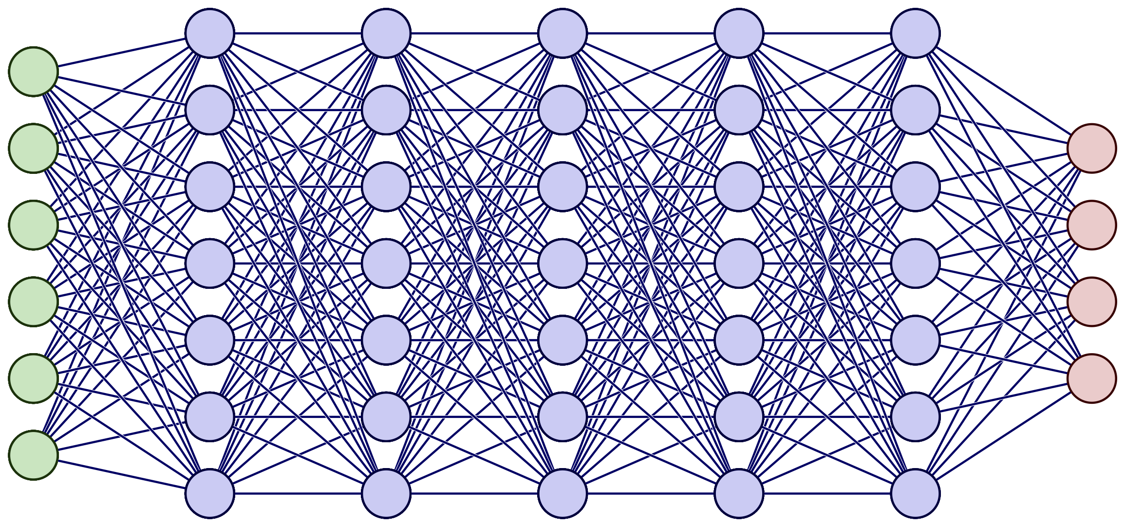A deep feedforward neural network. Image source

Convolutional Neural Networks (CNN)

CNNs specialize in image processing and are often used for image recognition tasks. They consist of several layers, including convolutional layers, pooling layers, and fully connected layers. The convolutional layers apply filters to the input images and extract features. The pooling layers reduce the size of the feature maps. Fully connected layers then classify the extracted features.

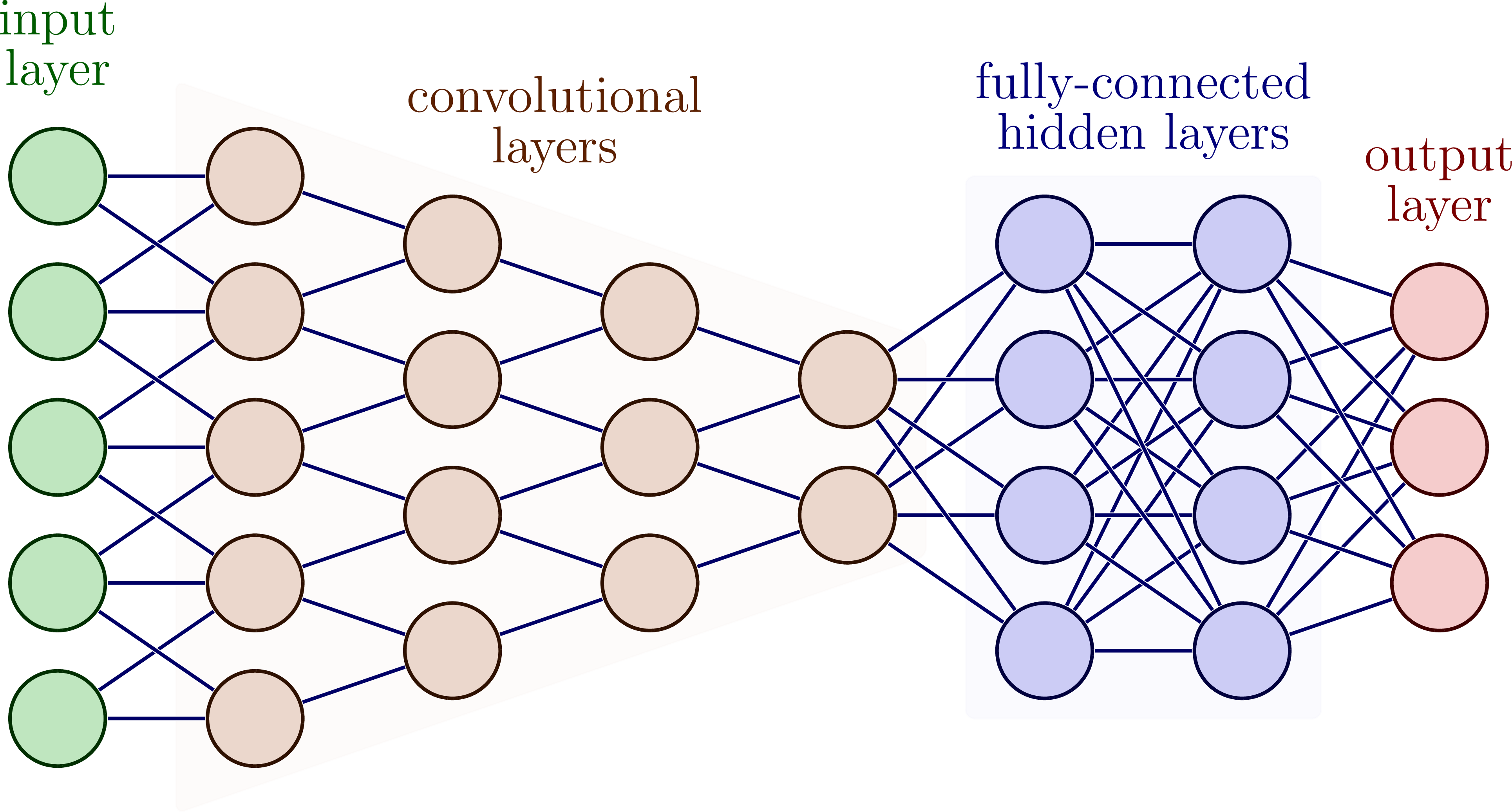A deep convolutional neural network with different layers. Image source

Recurrent Neural Networks (RNN)

RNNs specialize in processing sequences, such as speech and time series. They have an internal memory function that allows them to store information from previous steps and use it in future steps. RNNs consist of one or more layers connected to recurrent neurons.

Gradient descent method in 3-dimensional space. Image source

Long Short-Term Memory (LSTM) Networks

LSTMs are a type of RNN that are particularly well suited for processing long sequences. They have a complex architecture that allows them to store and forget information over the long term. LSTM networks are often used in speech recognition, text processing, and translation.

Gradient descent method in 3-dimensional space. Image source

Physical Guided Neural Network (PGNNs)

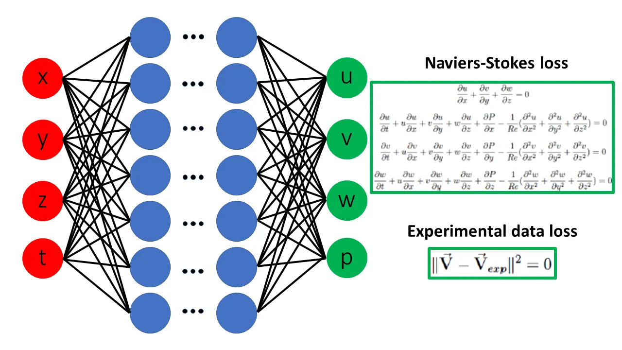
Another interesting concept is PGNN, also known as Physical Informed Neural Network (PINN). PGNNs use physical laws and mathematical models to predict the behavior of a system. They are often used in numerical simulation and process optimization to accelerate and optimize the design process. PGNNs require less training data than traditional machine learning models and can significantly reduce the cost and time required to conduct experiments. They are used in fluid dynamics, materials science, and engineering to simulate and optimize processes such as flow, heat transfer, and mechanical stress.

Gradient descent method in 3-dimensional space. Image source

Autoencoders

Autoencoders are a special type of neural network whose goal is to reconstruct the input data as accurately as possible. They consist of an encoder part, which maps the input data to a compressed latent space, and a decoder part, which transforms the data from this space back to the original input format.

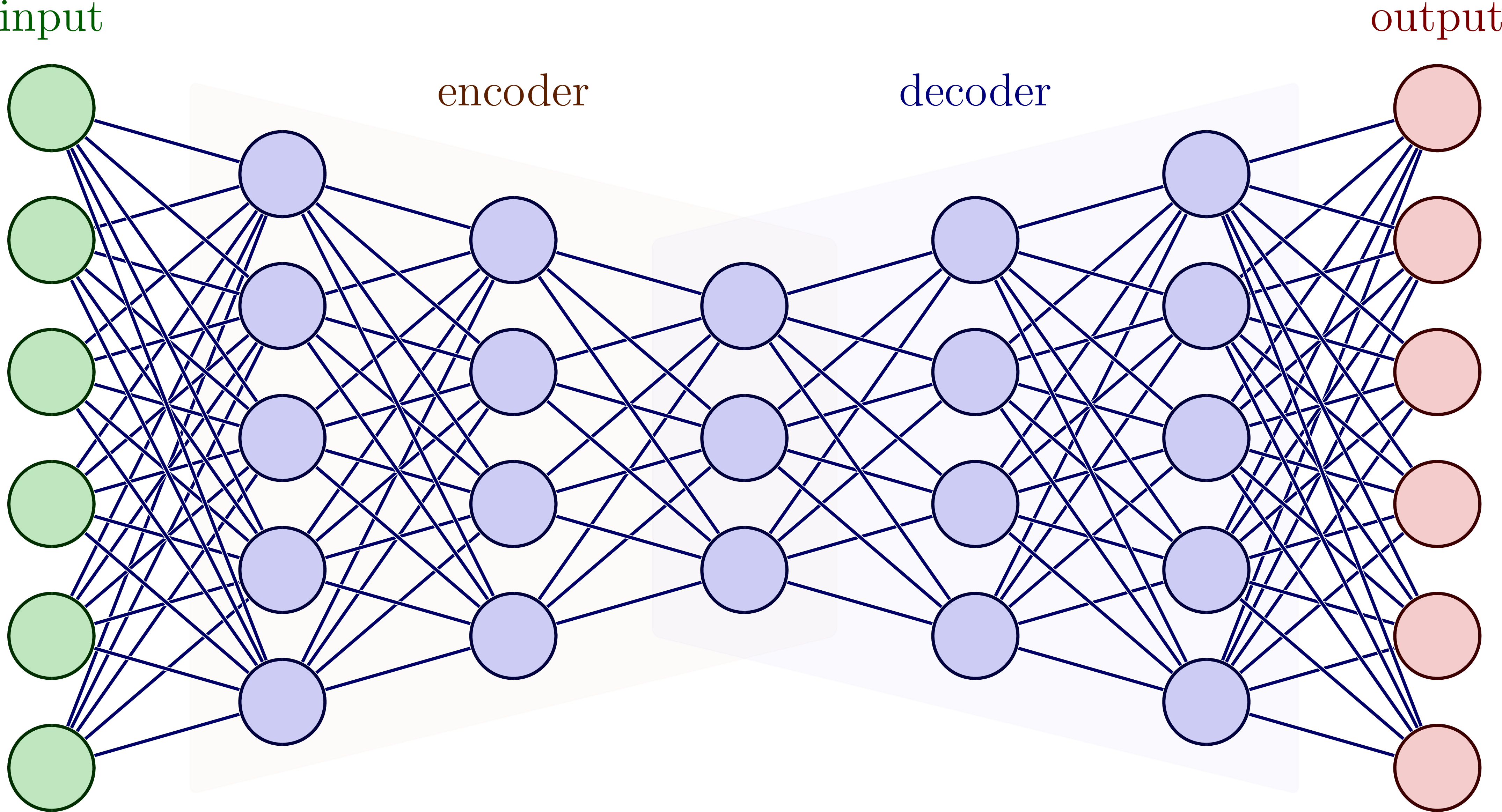An autoencoder network (encoder + decoder). Image source

Depending on the use case, different types of networks can be used to achieve the best possible result.

Summary

In this article, I hope I have been able to teach you something about neural networks: What is the Hello World! of machine learning? What does this so-called MNIST dataset look like in detail? What is a confusion matrix and how do neural networks learn? What are cost functions, backpropagation, optimizers, etc.?

I have also described a few of the activation functions and optimizers and shown a few types of neural networks.

If you have any questions or have found any errors, please feel free to contact me. In future posts, I would like to describe individual topics such as optimizers in more detail.

Digital garden

Explorer

Neural networks explained, using the MNIST example

How can you teach a computer to recognize a number? Or characters? Cell phone numbers? Signs?

The MNIST dataset

Overview of the MNIST dataset

Feature maps

The neural network

The neuron

One-hot encoding

Building the neural network

Underfitting, overfitting, and dropout

Confusion matrix

Training the neural network

Forward propagation

Error calculation: Cost functions

Backpropagation

Weight update

Summary

Activation Functions

Sigmoid function

Rectified Linear Unit (ReLU)

Tanh (hyperbolic tangent)

Optimizers

Stochastic Gradient Descent (SGD):

Adam (Adaptive Moment Estimation)

RMSProp (Root Mean Square Propagation)

Types of neural networks

Feedforward networks

Convolutional Neural Networks (CNN)

Recurrent Neural Networks (RNN)

Long Short-Term Memory (LSTM) Networks

Physical Guided Neural Network (PGNNs)

Autoencoders

Summary

Graph View

Table of Contents

Backlinks