The Decision Tree

In this article, I would like to discuss decision trees. Since it makes sense, we will also briefly talk about GridSearchCV and other necessary libraries. And all of this does not work - at least in my case - without Python. We will go through this Python code block by block/line by line. It is definitely advantageous if you have programmed before and ideal if you are familiar with Python

Decision Tree

Let’s start with the decision tree. Decision trees are used for both classification and regression tasks. The following graphic of a decision tree (which we will program below) shows the hierarchical sequence of decisions. This is a structured process for making decisions. Each node represents a decision, each edge a result or a subsequent decision.

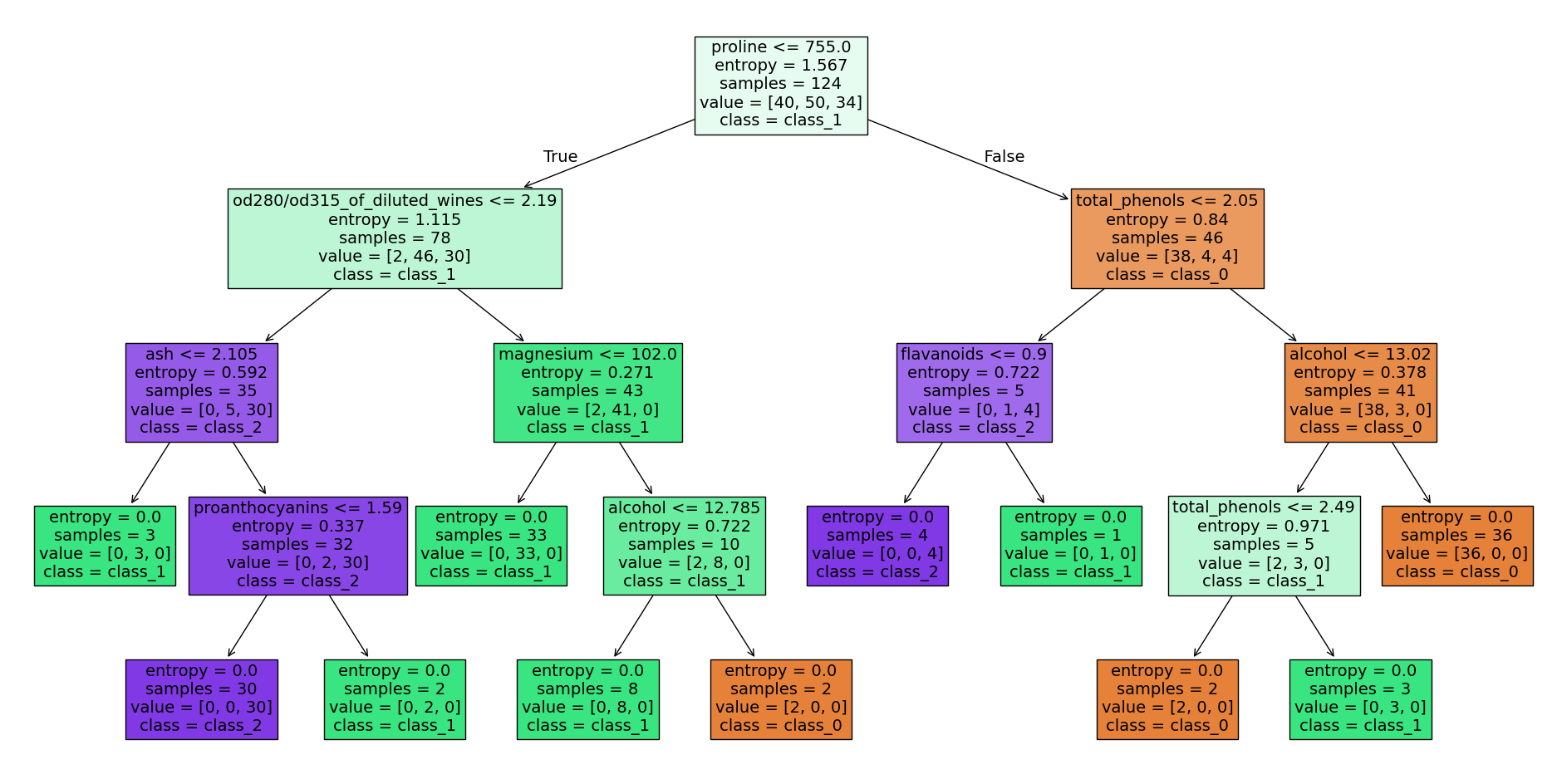Decision tree wine data set - source code at the end of the article, image by the author

A decision tree is a supervised learning algorithm.

The wine dataset

Let’s now dive into programming such a decision tree with the help of Scikit-learn’s wine dataset. First, we need to import the necessary libraries in Python:

import numpy as np
np.random.seed(42)
import pandas as pd
from sklearn.datasets import load_wine
from sklearn.tree import DecisionTreeClassifier
from sklearn.model_selection import GridSearchCV
from sklearn.model_selection import train_test_split

• Numpy is a program library that enables easy handling of vectors, matrices, and higher-dimensional arrays. It also offers a variety of functions for numerical calculations that are frequently used in scientific programming and data analysis.
• Pandas is a program library that facilitates the processing and analysis of tabular data. It provides data structures such as Series and DataFrame, which are similar to columns and tables in relational databases or arrays in Numpy. With pandas, you can easily read, edit, manipulate, model, and visualize data. It is one of the most commonly used tools in data analysis and preparation.
• The wine dataset (load_wine) is a sample dataset included in the Python library Scikit-learn. It contains information about various wines, such as alcohol content, acidity, color pigments, and proanthocyanidins. The dataset consists of 178 samples of wines and 13 features. This dataset is often used in examples to demonstrate the use of Scikit-learn for classification problems
• The DecisionTreeClassifier is a classification model from the Scikit-learn library based on the concept of a decision tree. The DecisionTreeClassifier creates a decision tree from the given training data and then uses it to classify new input data. This model is particularly useful for identifying patterns and relationships in complex, multidimensional data sets. It is easy to understand and interpret, and it is also robust to changes in the data.
• GridSearchCV is a method that allows you to try out a variety of hyperparameters for a given algorithm and automatically select the best parameters. GridSearchCV performs a search over a specified parameter range and estimates the performance of the algorithm using a specified evaluation function. It allows you to quickly and easily find the best hyperparameters for a model without having to try each value manually.
• train_test_split is a function used to split a dataset into training and test data. It takes the dataset and target variables as input and splits them into two parts: one part for training the model and one part for evaluating the model’s performance.

In the next code block, the wine dataset is first loaded and then the features data and the observation variables target of the wine dataset are assigned to x and y. This simply saves us a few keystrokes later on, and x and y are common names for precisely these data.

dataset = load_wine()
x, y = dataset.data, dataset.target

We then transfer the data to a Pandas DataFrame and assign the columns dataset.feature_names (the feature names) and y (the observation variable).

df = pd.DataFrame(x, columns = dataset.feature_names)
df["y"] = y
df.head()

With df.head(), you can now display the first 5 rows of the DataFrame and take a closer look at the dataset.

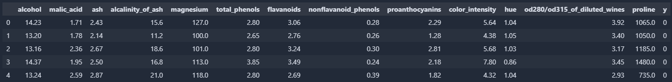df-head() of our DataFrame, image by the author

One of the features, for example, is the alcohol content in the first column. In column y, on the other hand, the class to be learned ($0$, $1$, or $2$) is stored. If you want to learn more about the features and the data set, you can find more information at this link to the Scikit-learn documentation. Once our DataFrame has been created and we have divided our data into x and y, we create training and test data sets.

x_train, x_test, y_train, y_test = train_test_split(
    x, y, test_size = 0.3, random_state=42)

The top line is used to split the data set consisting of x and y into randomly distributed training and test data sets using a seed (here random_state = 42). test_size = 0.3 defines that in this case the test data set should contain $30\%$ of the original wine data set.

• A seed refers to the starting value used to initialize a random number generator. This starting value determines the first random number generated by the generator, and the following random numbers are calculated using a deterministic algorithm based on the seed. If the same seed is used for multiple runs, the random number generator will generate the same series of random numbers. This can be advantageous for ensuring the reproducibility of experiments or for comparing the results of simulations.

In the next code block, the hyperparameters criterion, max_depth, min_samples_split, min_samples_leaf, and max_features are specified for GridSearchCV.

parameters = {
    'criterion': ['gini', 'entropy'],
    'max_depth': [None, 2, 4, 8, 10],
    'min_samples_split': [1, 2, 4], 
    'min_samples_leaf': [1, 2],
    'max_features': ['auto', 'sqrt', 'log2']
}

• criterion specifies which evaluation function should be used to evaluate the performance of the various models tested by GridSearchCV. Examples of possible criteria are accuracy, the logarithmic loss function, or the F1 score. By selecting the right criterion, you can ensure that the model is adapted to the specific requirements of the problem.
• max_depth specifies the maximum depth of the tree. It is used to find the optimal depth of the tree by trying different values and selecting the best results. A higher max_depth leads to more complex and potentially more adaptable models, but also to a higher risk of overfitting.
• min_samples_split is used to determine the minimum number of samples that must be present in a node before a split can be made. A higher value results in a deeper tree and may prevent overfitting. However, a lower value may result in a tree that is too shallow and may not be able to capture the relevant pattern recognition.
• min_samples_leaf is used to determine the number of samples per leaf in the decision tree. A higher value makes the leaves in the tree less sensitive to small changes in the data, thus preventing overfitting. However, a low value can cause the tree to become prone to overfitting and possibly unable to capture the relevant pattern recognition.
• max_features is used to determine the number of features to consider at each split. There are three ways to set the value: as an absolute value (e.g., max_features = 4), as a fraction of the available features (e.g., max_features = 0.8), or as a logarithmic fraction of the available features (e.g., max_features = log2). A higher value causes the tree to consider more features, which allows it to capture more complex pattern recognition, but can also lead to overfitting. A low value can cause the tree to be unable to capture the relevant pattern recognition.

If you want to learn more about GridSearchCV, check out the Scikit-Learn documentation. Now we’ll finally create an instance of the DecisionTreeClassifier, or our first decision tree, and initialize the GridSearchCV before we run it. Depending on your computer’s performance, this process may take a while.

clf = DecisionTreeClassifier()
grid_cv = GridSearchCV(clf, parameters, cv = 10, n_jobs = -1)
grid_cv.fit(x_train, y_train)

GridSearchCV now tries every combination of the parameters defined above and uses the score to determine the best combination of hyperparameters. cv = 10 means that our data set is divided into ten equal parts (folds). The model is then trained on nine parts and validated on the tenth part. This process is repeated ten times, with the part to be validated changing each time. n_jobs = -1 allows the use of all CPUs, thus speeding up the process. After training (fit), we output these hyperparameters

print(f"Parameters of best model: {grid_cv.best_params_}")
print(f"Score of best model: {grid_cv.best_score_}")

The result of the GridSearchCV search. The score describes the performance of the model:

Parameters of best model: {'criterion': 'gini', 'max_depth': 4, 'max_features': 'log2', 'min_samples_leaf': 1, 'min_samples_split': 2}
Score of best model: 0.9589743589743589

We incorporate these parameters into our decision tree and train it.

clf = DecisionTreeClassifier(
    criterion='gini', 
    max_depth=10, 
    max_features='sqrt', 
    min_samples_leaf=1, 
    min_samples_split=2)
clf.fit(x_train, y_train)

During this iterative process, our decision tree is continuously adjusted and improved. Once we have completed our training, we can test the performance of our tree on the test data.

score = clf.score(x_test, y_test)
print(f"Accuracy: {score}")

Accuracy: 0.8703703703703703

The score of a decision tree refers to the performance of the model as measured by a specific metric. The most common metric used to measure the performance of a decision tree is accuracy. It indicates how often the model predicted the correct class for a given example. It is calculated as the number of correctly classified examples divided by the total number of examples. It is important to note that accuracy alone is not always a sufficient measure of a decision tree’s performance, especially if the classes in the dataset are unevenly distributed or if the model needs to be able to minimize certain types of errors. In such cases, other metrics, such as precision, recall, or F1 score, may be more useful.

Our decision tree can also be represented graphically. The following lines import the necessary libraries and ultimately map the decision tree with the decisions, etc.

from sklearn import tree
import graphviz
dot_data = tree.export_graphviz(clf, out_file=None, 
                                feature_names=dataset.feature_names,  
                                class_names=dataset.target_names,
                                filled=True)
graph = graphviz.Source(dot_data, format="png") 
graph

The lines above provide the decision tree at the beginning of this post. If you have any questions, please feel free to contact me.

The following code prints in text, what is shown in picture above.

from sklearn.tree import export_text
 
tree_rules = export_text(clf, feature_names=dataset.feature_names)
print(tree_rules)

|--- proline <= 755.00
|   |--- od280/od315_of_diluted_wines <= 2.19
|   |   |--- ash <= 2.11
|   |   |   |--- class: 1
|   |   |--- ash >  2.11
|   |   |   |--- proanthocyanins <= 1.59
|   |   |   |   |--- class: 2
|   |   |   |--- proanthocyanins >  1.59
|   |   |   |   |--- class: 1
|   |--- od280/od315_of_diluted_wines >  2.19
|   |   |--- magnesium <= 102.00
|   |   |   |--- class: 1
|   |   |--- magnesium >  102.00
|   |   |   |--- alcohol <= 12.78
|   |   |   |   |--- class: 1
|   |   |   |--- alcohol >  12.78
|   |   |   |   |--- class: 0
|--- proline >  755.00
|   |--- total_phenols <= 2.05
|   |   |--- flavanoids <= 0.90
|   |   |   |--- class: 2
|   |   |--- flavanoids >  0.90
|   |   |   |--- class: 1
|   |--- total_phenols >  2.05
|   |   |--- alcohol <= 13.02
|   |   |   |--- total_phenols <= 2.49
|   |   |   |   |--- class: 0
|   |   |   |--- total_phenols >  2.49
|   |   |   |   |--- class: 1
|   |   |--- alcohol >  13.02
|   |   |   |--- class: 0

Summary

At this point, we have now used our first data set and programmed our first decision tree. We have also looked at what GridSearchCV does, for example, and why it can be so useful for us.

In the next article, I will describe what a random forest is and how to program it.