The Random Forrest

In the last article, I described what a decision tree is. It is a structured process for making decisions. Decision trees are often used for classification or regression procedures. In this article, I would like to show you what a random forest is. We will once again dive into Python code. This also means that I have again made the source code available to you in the GitHub repository.

The Random Forest

A random forest consists of several uncorrelated decision trees. Each of these decision trees was created during the learning process under a specific randomization and was trained with random subsets of the initial data. The final prediction of the model is determined by coordinating the predictions of all decision trees. This increases the prediction accuracy and makes the model more robust against overfitting. For example, if we try to solve a classification problem, each tree in the forest is allowed to make a decision, and a majority vote is taken, so to speak: the most frequently selected class determines the final classification. Random forests can also be used for regression problems. As with decision trees, a random forest is also an algorithm of supervised learning. In addition, a random forest is a so-called ensemble model.

• An ensemble model is a machine learning method in which multiple models are combined to increase prediction accuracy.

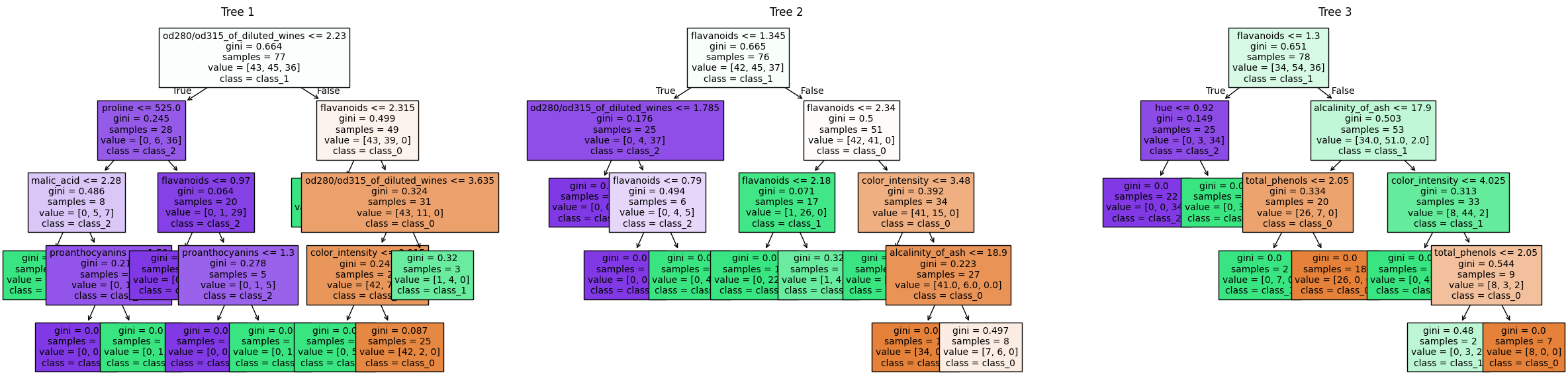Random Forest (Ensemble Model) with three estimators

The image above shows three decision trees from the programmed random forest. The source code for the random forest follows in the next section.

The program code

Some of the following lines should already be familiar from the previous article on decision trees. For this reason, I will summarize some lines/blocks and only describe them briefly. I will, of course, go into more detail on any special features.

from sklearn.datasets import load_wine
from sklearn.ensemble import RandomForestClassifier
from sklearn.model_selection import GridSearchCV
from sklearn.model_selection import train_test_split

The imports are the same as for the decision tree. For comparison purposes, we will again use the wine data set.

dataset = load_wine()
x, y = dataset.data, dataset.target
x_train, x_test, y_train, y_test = train_test_split(
  x, y, test_size = 0.3, random_state = 42)

This is followed by the division into training and test data sets.

parameters = {
    'criterion': ['gini', 'entropy'],
    'max_depth': [None, 2, 4, 8, 10],
    'min_samples_split': [2, 4],
    'min_samples_leaf': [1, 2],
    'max_features': ['auto', 'sqrt', 'log2'],
    'n_estimators': [10, 20, 50, 100, 200]
}

The hyperparameters for GridSearchCV are defined in the code block above. These are largely the same as for the decision tree. However, I have added n_estimators.

• n_estimators is a hyperparameter in Random Forest and specifies the number of decision trees to be used. A higher value of n_estimators usually leads to better results, but it can also take longer to train the model. It is a trade-off between prediction accuracy and training time

clf = RandomForestClassifier(random_state = 42)
grid_cv = GridSearchCV(clf, parameters, cv = 10, n_jobs = -1)
grid_cv.fit(x_train, y_train)

Similar to the decision tree, the classifier - now the RandomForestClassifier - is instantiated and the GridSearchCV is initialized and executed. The results are provided by the following code block:

print(f"Parameters of best model: {grid_cv.best_params_}")
print(f"Score of best model: {grid_cv.best_score_}")

Parameters of best model: {'criterion': 'gini', 'max_depth': 4, 'max_features': 'sqrt', 'min_samples_leaf': 1, 'min_samples_split': 4, 'n_estimators': 20}
Score of best model: 0.9839743589743589

These are the best hyperparameters according to the above GridSearchCV. With n_estimators = 20 and thus $20$ individual decision trees, we achieve a score of $\mathrm{0.98...}$ As a reminder, the score of a single decision tree from the previous article is $\mathrm{0.95...}$

And if you now apply the trained model to the test data, you get a score of $\mathrm{0.94...}$

score = grid_cv.score(x_test, y_test)
print(f"Accuracy: {score}")

Accuracy: 0.9444444444444444

And again, here is a comparison with the single decision tree. This delivered an accuracy of $\mathrm{0.88...}$

The higher accuracy of a random forest compared to a single decision tree mentioned at the beginning could therefore be confirmed, at least for this data set.

For completeness, here is the visualization of all $20$ estimators.

Complete random forest

Summary

In the sections above, we learned what a random forest is and how to program it with Sklearn. We tried to stay as close as possible to the decision tree from the previous article so that we could compare the results.