Theory and formulas behind the decision tree

In the last two articles, we learned how to program decision trees and random forests. This article will focus on the theory behind them. But first, a quick recap.

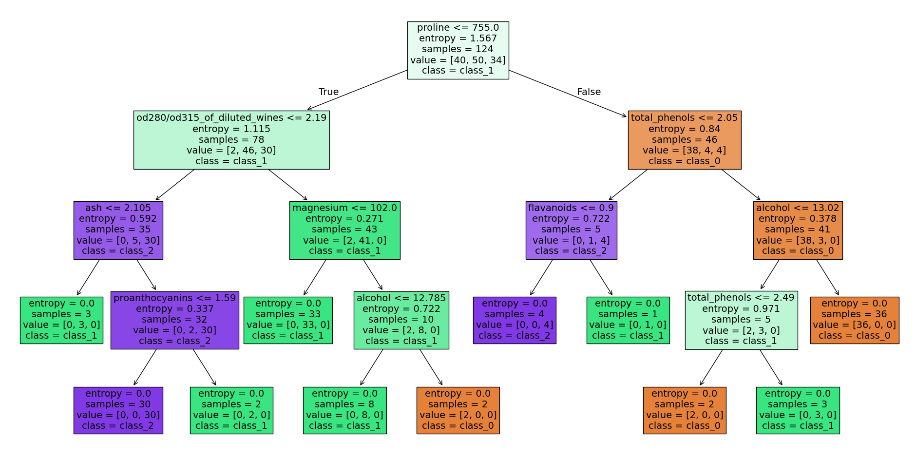Decision tree wine dataset - source code at the end of the article

Decision trees are a well-known model in machine learning and are often used for classification and regression problems. They represent a hierarchy of decisions and predictions based on specific features and rules.

A random forest, on the other hand, consists of several uncorrelated decision trees that were created during the learning process under a certain randomization and trained with random subsets of the input data. The final prediction of the model is determined by averaging the predictions of all decision trees.

But now let’s move on to the concepts and theory behind decision trees and, ultimately, random forests.

Information Gain and Entropy

One of the most important concepts in decision trees is Information Gain. This is a measure that determines which feature is best suited to split the data. The Information Gain is calculated by determining the difference between the original entropy value and the entropy value after the split.

Entropy

The entropy value measures the disorder or heterogeneity of a group of observations. A higher entropy means a higher disorder and a lower prediction accuracy. The entropy value is calculated by logarithmically calculating and summing the probability of each class in the group.

The entropy of a discrete random variable $X$ with possible outcomes $x_1,x_2,\dots ,x_n$ and probabilities $p_1,p_2,\dots ,p_n$ is defined as:

$H(X)=-{\sum }_{i=1}^N{P}_i\cdot lo{g}_2(P_i)$

Information Gain

Information Gain is calculated by determining the difference between the original entropy value and the entropy value after the split. For example, if we split a group of observations based on a specific feature, like age, and it’s a good splitting feature, the observations will be divided into clearer and more homogeneous groups, which leads to lower entropy. The information gain is then the difference between the original entropy value and the entropy value after the split.

The Information Gain, which depends on a decision A and reflects the difference in entropy before and after the decision, is defined as:

$IG(A)=H(S)-\sum p(t)\cdot H(t)$

where $S$ is the set of all examples to be decided, $t$ is the set of examples where decision $A$ was made, $p(t)$ is the probability that an example is in $t$, and $H(t)$ is the entropy of $t$.

In other words, Information Gain measures how much entropy is reduced when a specific decision is made, compared to the entropy of the original set of examples. A high information gain means that a decision is more useful because it reduces more entropy and thus provides more information.

Gini impurity

Gini impurity is a measure of the impurity of a set of data. It is used in decision tree classification to evaluate the quality of splits in the data. Gini impurity measures how often a randomly selected element in the set would be misclassified if it were classified randomly according to the distribution of classes in the set. A value of $0$ means that the set is completely pure (all elements have the same class), while a value of $1$ means that the set is completely impure (the elements are evenly distributed across the classes). Gini impurity can be calculated as follows. $Gini=1-{\sum }_{i=1}^n(p_i{)}^2$ $n$ is the number of classes and $p_i$ is the relative frequency of instances of class $i$ in the split. When calculating Gini impurity, it is assumed that each split contains at least one instance of each class. If a split does not contain any instances of a particular class, the Gini impurity is $0$, which means that the split provides perfect class separation. The choice between using information gain or Gini impurity often depends on the specific requirements and preferences of the user. Information gain is a well-known metric and provides a clear mathematical basis, but Gini impurity can be calculated more quickly and is easier to interpret in some cases. In summary, Gini impurity calculates the impurity of a particular split in a decision tree and is an important indicator of prediction accuracy. The lower the Gini impurity, the better the class separation and the higher the prediction accuracy.

Overfitting

Another important concept or problem with decision trees is overfitting. This occurs when a model is too complex and is overly adapted to the training data instead of making general predictions. Overfitting can lead to poor prediction accuracy on new, unseen data. There are several techniques that can prevent overfitting in decision trees:

1. Pruning: This technique involves pruning the tree after it has been created to remove unnecessarily complex structures. There are two main types of pruning: reduced error pruning and cost complexity pruning.
2. Minimizing the number of leaves: Another way to avoid overfitting is to minimize the number of leaves. This can be achieved by increasing the threshold or by applying rules to merge leaves.
3. Use of ensembles: A combination of several decision trees trained on different training data can improve prediction accuracy and reduce overfitting. The best-known methods are bagging and boosting.
4. Use of regularization terms: It is possible to use regularization terms such as $L1$ and $L2$ to reduce the influence of certain variables on the decision-making process and thus prevent overfitting.
5. Data augmentation: Another approach is to augment the data by artificially generating new data points that are similar to the existing ones. This can help reduce variance and overfitting. It is important to note that there is no single method for avoiding overfitting and that the choice of method depends on the specific problem. If you are interested in learning more about this topic, let me know and I will prepare more information.

Summary

In summary, decision trees are a powerful method in machine learning and are based on information gain, Gini impurity, overfitting, and stopping conditions. Although they are not suitable for every problem, they are an important part of every data scientist’s toolbox.